Bayesian Networks

Caution

Metrics and analyses for the regional secondary data project are works in progress. There are some metric cleanliness issues here that I’m putting off for now until we work back through the county metrics.

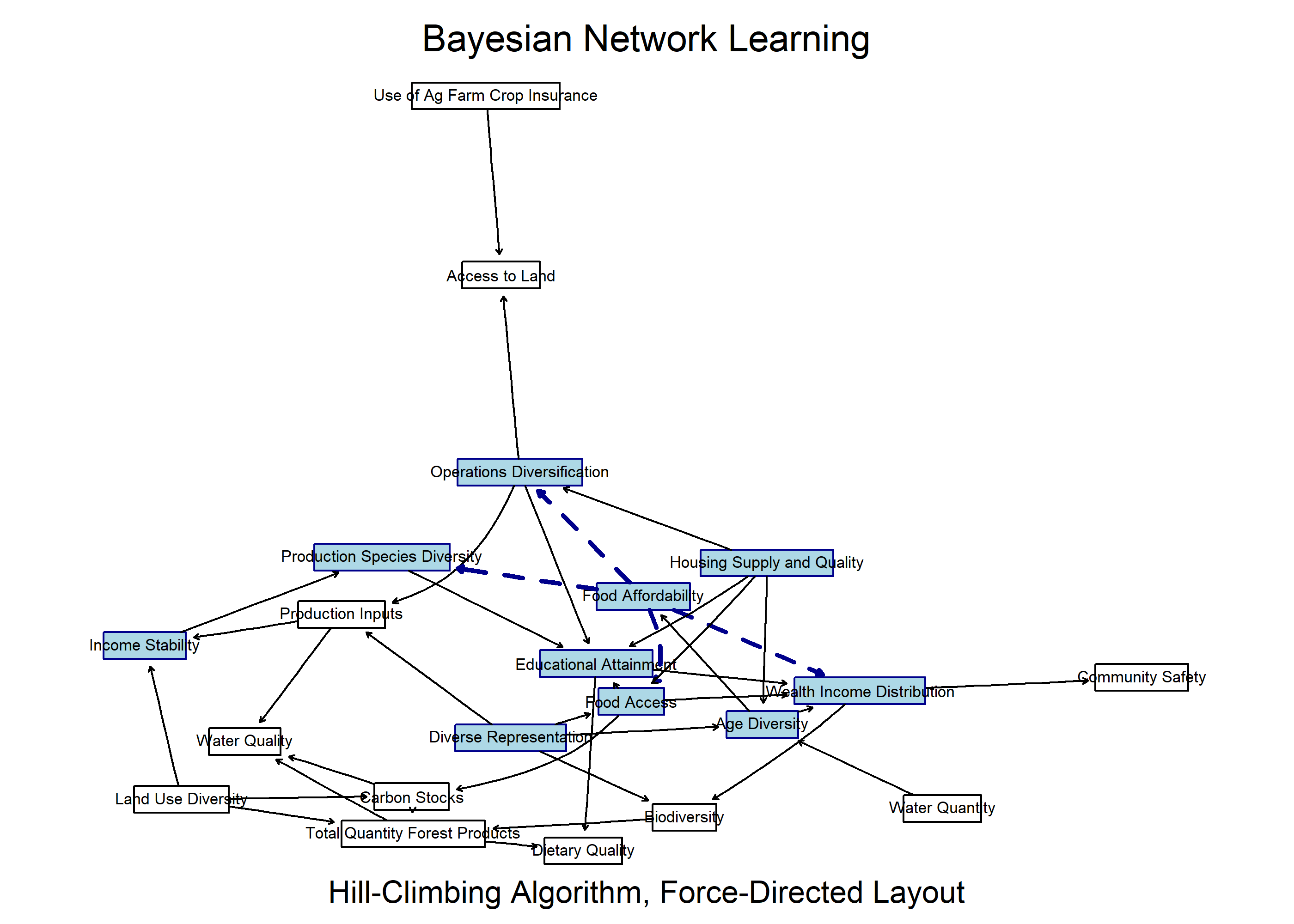
Testing out a Bayesian Network with structural learning to identify drivers in our food systems data.

Strengths:

Causal inference from observational data, with assumptions:
- Causal Markov assumption
- Faithfulness
- Causal sufficiency
Structural and parameter learning
Forward and backward inference
Whitelisting and blacklisting allows for hybrid model that combines priors with observed data, making it quite effective in low-data scenarios

Drawbacks:

Cannot model feedback loops or thresholds (i.e., no complex systems)
No particularly convincing way to approach dynamic models, although some options exist

1 Housekeeping

Code

# if (!require('graph')) BiocManager::install('graph')
# if (!require('Rgraphviz')) BiocManager::install('Rgraphviz')

pacman::p_load(
  dplyr,
  bnlearn,
  conflicted,
  stringr,
  purrr,
  tidyr,
  skimr,
  knitr,
  reactable,
  graph,
  Rgraphviz,
  snakecase,
  graph
)

source('dev/data_pipeline_functions.R')
source('dev/get_reactable.R')

conflicted::conflicts_prefer(
  dplyr::filter(),
  dplyr::select(),
  base::setdiff(),
  base::intersect(),
  base::union(),
  igraph::degree(),
  bnlearn::score(),
  graph::nodes(),
  .quiet = TRUE
)

2 Wrangling

Code

# Pull county time series variables
vars <- readRDS('data/frontiers/county_time_series_vars.rds')
sm_data <- readRDS('data/sm_data.rds')[['metrics']]

# Get county variables only, and lose CT
dat <- sm_data %>% 
  filter(
    str_length(fips) == 5,
    variable_name %in% vars,
    value != -666666666,
    str_detect(fips, '^09', negate = TRUE)
  ) %>% 
  mutate(across(c(year, value), ~ as.numeric(.x)))
get_str(dat)

# Get latest year only, then pivot wider for analysis
dat <- dat %>% 
  get_latest_year(add_suffix = FALSE) %>% 
  pivot_wider(
    id_cols = fips,
    values_from = value,
    names_from = variable_name
  )
get_str(dat)

# Check missing
(skim_out <- skim(dat))

# Ditch vars that are > 50% missing
mis <- skim_out %>% 
  filter(complete_rate < 0.5) %>% 
  pull(skim_variable)
dat <- select(dat, -any_of(mis))
get_str(dat)
# Noice

3 State Data

Let’s try this with our aggregated indicators from national data at state level. County data for regional level are still in progress. We are also mostly poking around with the hill-climbing algorithm at this point, which is greedy and tends to draw more paths than other methods. This should be refined as we move along the process.

3.1 Preprocessing

Code

scores <- readRDS('data/raw_minmax_geo.rds')
get_str(scores)
df <- scores %>% 
  select(matches('^indic')) %>% 
  setNames(c(str_remove(names(.), 'indic_') %>% str_replace_all(' ', '_')))
get_str(df)

# Get rid of county, also FFF variables
# get_str(dat)
# df <- dat %>% 
#   select(-any_of(c('fips', matches('FFF$'))))
# get_str(df)

# Remove highly correlated variables
threshold <- 0.5
df <- dedup(df, threshold = threshold)
names(df) <- snakecase::to_title_case(names(df))

Threshold of correlations at 0.5 brings us down from 66 variables to 21 variables.

3.2 Structural Learning

Run a series of different models to compare

Code

models <- list(
  dag_pc = pc.stable(df),
  dag_gs = gs(df),
  dag_iamb = iamb(df),
  dag_inter_iamb = inter.iamb(df),
  dag_hc = hc(df),
  dag_mmhc = mmhc(df)
)
# map(models, ~ try(score(.x, df)))

Plot one, highlighting the Markov blanket for food affordability.

Code

graphviz.plot(
  models$dag_hc,
  layout = 'fdp',
  shape = 'rectangle',
  fontsize = 24,
  main = 'Bayesian Network Learning',
  sub = 'Hill-Climbing Algorithm, Force-Directed Layout',
  highlight = list(
    nodes = rbind('Food Affordability', mb(models$dag_hc, 'Food Affordability')),
    arcs = outgoing.arcs(models$dag_hc, "Food Affordability"),
    fill = 'lightblue',
    col = "darkblue",
    lwd = 2.5,
    lty = 'dashed'
  )
)

3.3 Parameter Learning

Code

(fitted <- bn.fit(models$dag_hc, df))

Bootstrap how many arcs we get:

Code

unlist(bn.boot(df, statistic = narcs, algorithm = "hc", R = 10))

 [1] 55 60 58 64 61 53 53 55 55 56

Dummy models:

Code

bn.boot(df, statistic = function(x) x, algorithm = "hc", R = 2)

[[1]]

  Bayesian network learned via Score-based methods

  model:
   [Access to Land][Operations Diversification|Access to Land]
   [Income Stability|Operations Diversification]
   [Production Inputs|Operations Diversification]
   [Production Species Diversity|Income Stability]
   [Diverse Representation|Production Inputs]
   [Land Use Diversity|Production Species Diversity:Production Inputs]
   [Housing Supply and Quality|Operations Diversification:Production Species Diversity]
   [Use of Ag Farm Crop Insurance|Access to Land:Land Use Diversity]
   [Carbon Stocks|Land Use Diversity]
   [Dietary Quality|Carbon Stocks:Land Use Diversity]
   [Water Quality|Access to Land:Carbon Stocks:Dietary Quality:Production Inputs]
   [Total Quantity Forest Products|Operations Diversification:Land Use Diversity:Water Quality:Production Species Diversity]
   [Community Safety|Total Quantity Forest Products]
   [Biodiversity|Use of Ag Farm Crop Insurance:Total Quantity Forest Products:Community Safety]
   [Wealth Income Distribution|Income Stability:Operations Diversification:Biodiversity:Land Use Diversity:Housing Supply and Quality:Total Quantity Forest Products]
   [Food Access|Access to Land:Income Stability:Operations Diversification:Use of Ag Farm Crop Insurance:Carbon Stocks:Biodiversity:Dietary Quality]
   [Educational Attainment|Access to Land:Wealth Income Distribution:Use of Ag Farm Crop Insurance:Carbon Stocks:Food Access]
   [Food Affordability|Wealth Income Distribution:Food Access:Production Species Diversity:Diverse Representation]
   [Age Diversity|Biodiversity:Educational Attainment:Food Access:Housing Supply and Quality:Diverse Representation]
   [Water Quantity|Operations Diversification:Land Use Diversity:Total Quantity Forest Products:Age Diversity]
  nodes:                                 21 
  arcs:                                  57 
    undirected arcs:                     0 
    directed arcs:                       57 
  average markov blanket size:           10.48 
  average neighbourhood size:            5.43 
  average branching factor:              2.71 

  learning algorithm:                    Hill-Climbing 
  score:                                 BIC (Gauss.) 
  penalization coefficient:              1.956012 
  tests used in the learning procedure:  1429 
  optimized:                             TRUE 


[[2]]

  Bayesian network learned via Score-based methods

  model:
   [Use of Ag Farm Crop Insurance][Carbon Stocks][Water Quantity]
   [Land Use Diversity|Use of Ag Farm Crop Insurance:Carbon Stocks]
   [Production Inputs|Use of Ag Farm Crop Insurance]
   [Diverse Representation|Production Inputs]
   [Food Access|Carbon Stocks:Diverse Representation]
   [Age Diversity|Diverse Representation]
   [Housing Supply and Quality|Food Access:Age Diversity]
   [Income Stability|Land Use Diversity:Housing Supply and Quality:Production Inputs]
   [Dietary Quality|Housing Supply and Quality]
   [Production Species Diversity|Income Stability:Housing Supply and Quality]
   [Operations Diversification|Housing Supply and Quality:Production Species Diversity:Production Inputs]
   [Access to Land|Operations Diversification:Use of Ag Farm Crop Insurance:Diverse Representation]
   [Wealth Income Distribution|Income Stability:Operations Diversification:Use of Ag Farm Crop Insurance:Food Access:Housing Supply and Quality:Age Diversity]
   [Food Affordability|Operations Diversification:Age Diversity]
   [Total Quantity Forest Products|Wealth Income Distribution]
   [Community Safety|Wealth Income Distribution:Dietary Quality:Diverse Representation:Age Diversity]
   [Educational Attainment|Operations Diversification:Water Quantity:Food Access:Housing Supply and Quality:Production Species Diversity:Total Quantity Forest Products]
   [Water Quality|Access to Land:Operations Diversification:Carbon Stocks:Land Use Diversity:Water Quantity:Educational Attainment:Production Species Diversity:Total Quantity Forest Products]
   [Biodiversity|Wealth Income Distribution:Use of Ag Farm Crop Insurance:Water Quality:Housing Supply and Quality:Production Species Diversity:Community Safety:Diverse Representation]
  nodes:                                 21 
  arcs:                                  55 
    undirected arcs:                     0 
    directed arcs:                       55 
  average markov blanket size:           11.05 
  average neighbourhood size:            5.24 
  average branching factor:              2.62 

  learning algorithm:                    Hill-Climbing 
  score:                                 BIC (Gauss.) 
  penalization coefficient:              1.956012 
  tests used in the learning procedure:  1510 
  optimized:                             TRUE

Arc strength: confidence in a particular graphical feature of network. Bootstraps network, then estimates relative frequency of parameter of interest. Gets strength of every possible arc. Strength shows probability of the arc existing, Direction shows probability of it being the direction shown.

Code

arc_str <- boot.strength(df, algorithm = "hc")
get_reactable(arc_str)

Check the arc strengths for food affordability:

Code

arc_str %>% 
  filter(from == 'Food Affordability') %>% 
  get_reactable()

4 Things to Add

Hybrid structural learning algorithms (MMHC)
Whitelisting and blacklisting
Add covariates (no omitted variables)
Pair with fuzzy cognitive mapping