Here we will use the raw + min max + geometric aggregation scores and see how they hold up to validation by external variables and by PCA.
External variables:
Food Security Index (Feeding America, Map the Meal Gap)
Life expectancy, or premature age-adjusted mortality (UW County Health Rankings)
Food Environment Index (UW County Health Rankings)
Happiness Score (WalletHub - if anyone knows of a better metric for this, I’m all ears)
Code
# Load sm_datasm_data <-readRDS('data/sm_data.rds')# Load state fips key to join other datasetsstate_key <- sm_data[['state_key']] %>%select(state, state_code)# Load cleaned aggregated data for all levels of regresionraw_minmax_geo <-readRDS('data/raw_minmax_geo.rds')get_str(raw_minmax_geo)# Reduce to just dimension scores, and remove prefixdimension_scores <- raw_minmax_geo %>%select(state, starts_with('dimen')) %>%setNames(c(str_remove(names(.), 'dimen_')))get_str(dimension_scores)# Pull validation variables out of sm_data, wrangle them to match metrics_df# Also including covariates, gdp and populationvalidation_vars <- sm_data$metadata %>%select(variable_name, metric, definition, source) %>%filter(variable_name %in%c('foodInsecurity','communityEnvRank','happinessScore','wellbeingRank','workEnvRank','foodEnvironmentIndex','lifeExpectancy','population','gdpCurrent' )) %>%pull(variable_name)validation_vars # Get subset of metrics for our validation variables, get latest year onlyvalidation_metrics <- sm_data$metrics %>%filter( variable_name %in% validation_vars, !is.na(value), str_length(fips) ==2 ) %>%get_latest_year()get_str(validation_metrics)# All are available in 2024# Pivot wider, also get rid of trailing yearvalidation_metrics <- validation_metrics %>%pivot_wider(id_cols = fips,names_from = variable_name,values_from = value ) %>%setNames(c(str_remove(names(.), '_[0-9]{4}'))) %>%mutate(across(!fips, as.numeric))get_str(validation_metrics)# 00 US is missing a lot obviously# 11 DC is the other one with missing data# We will just filter down to 50 states to match metrics_df# Combine validation variables with our dimension scores using state key as the # bridge. Also remove DC (don't have validation metrics there)key <- sm_data$state_key %>%select(state, fips = state_code)dat <- dimension_scores %>%left_join(key) %>%left_join(validation_metrics) %>%as.data.frame() %>%filter(state !='DC') %>%select(-fips)# Make a GDP per capita variable from GDP real and population# It was already in millions to begin withdat <- dat %>%mutate(gdp_per_cap = ((gdpCurrent / population) *1e6) /1000)get_str(dat)# Check it outget_str(dat)skimr::skim(dat)# Looks good# Save this for other pagessaveRDS(dat, 'data/metrics_df_with_vals_and_covars.rds')
2 Regression
2.1 Food Insecurity
Code
lm1 <-lm( foodInsecurity ~ economics + environment + health + production + social,data = dat)
Dependent variable:
Food Insecurity Index
Dimensions Only
With GDP per Capita
GDP and Pop. Weights
(1)
(2)
(3)
Constant
0.157*** (0.126, 0.188)
0.162*** (0.123, 0.202)
0.163*** (0.128, 0.199)
economics
-0.002 (-0.072, 0.069)
-0.005 (-0.077, 0.068)
-0.038 (-0.103, 0.027)
environment
0.062 (0.001, 0.122)
0.059 (-0.003, 0.121)
0.034 (-0.025, 0.094)
health
-0.185*** (-0.257, -0.112)
-0.175*** (-0.260, -0.089)
-0.187*** (-0.270, -0.103)
production
-0.012 (-0.058, 0.033)
-0.011 (-0.057, 0.036)
0.014 (-0.013, 0.041)
social
0.012 (-0.058, 0.083)
0.011 (-0.061, 0.083)
-0.007 (-0.069, 0.055)
gdp_per_cap
-0.0001 (-0.001, 0.0003)
0.0002 (-0.0002, 0.001)
WLS
No
No
Yes
Robust
No
No
No
Observations
50
50
50
R2
0.546
0.548
0.629
Adjusted R2
0.494
0.485
0.578
Residual Std. Error
0.017 (df = 44)
0.017 (df = 43)
32.875 (df = 43)
F Statistic
10.574*** (df = 5; 44)
8.679*** (df = 6; 43)
12.166*** (df = 6; 43)
Note:
⋆p<0.05; ⋆⋆p<0.01; ⋆⋆⋆p<0.001
Code
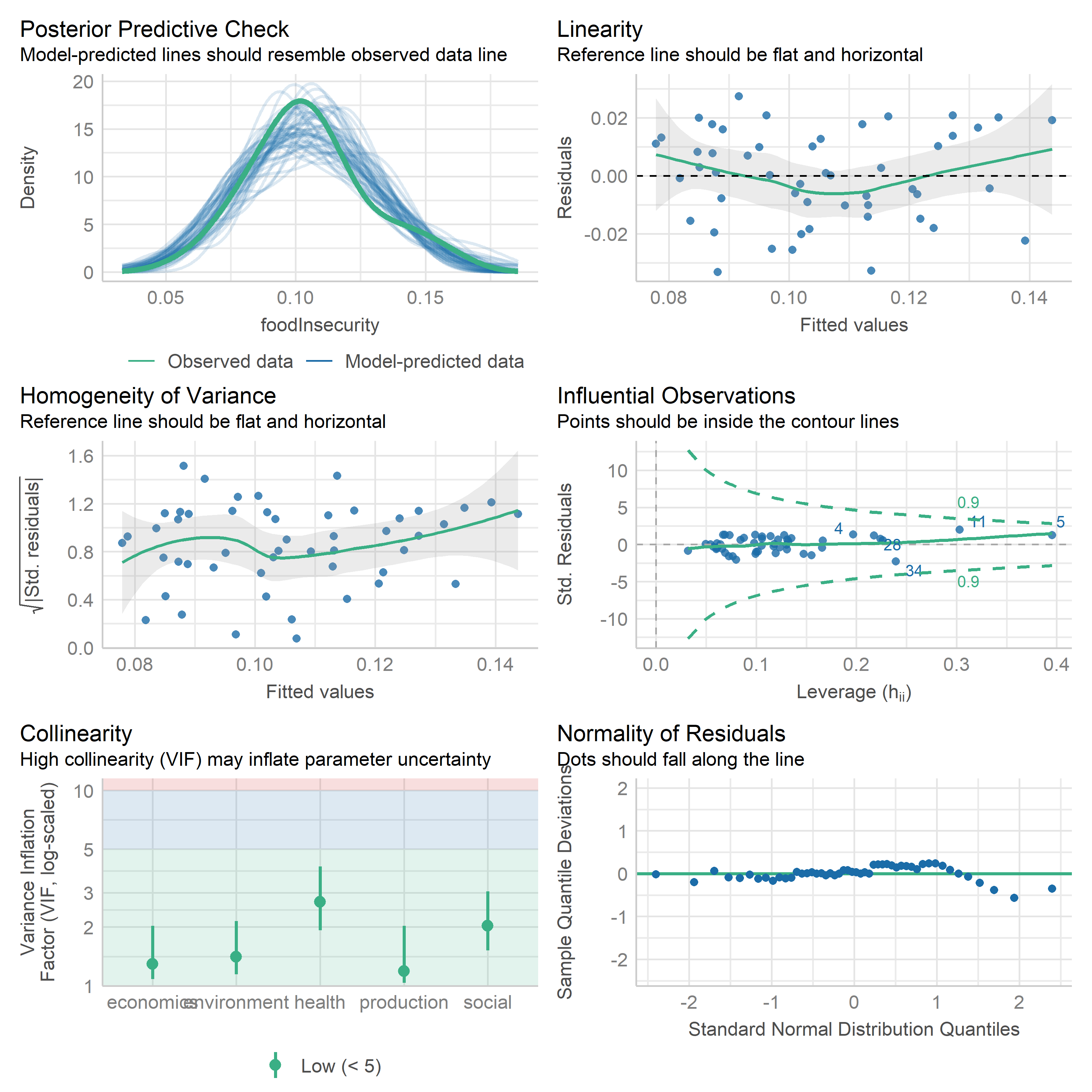
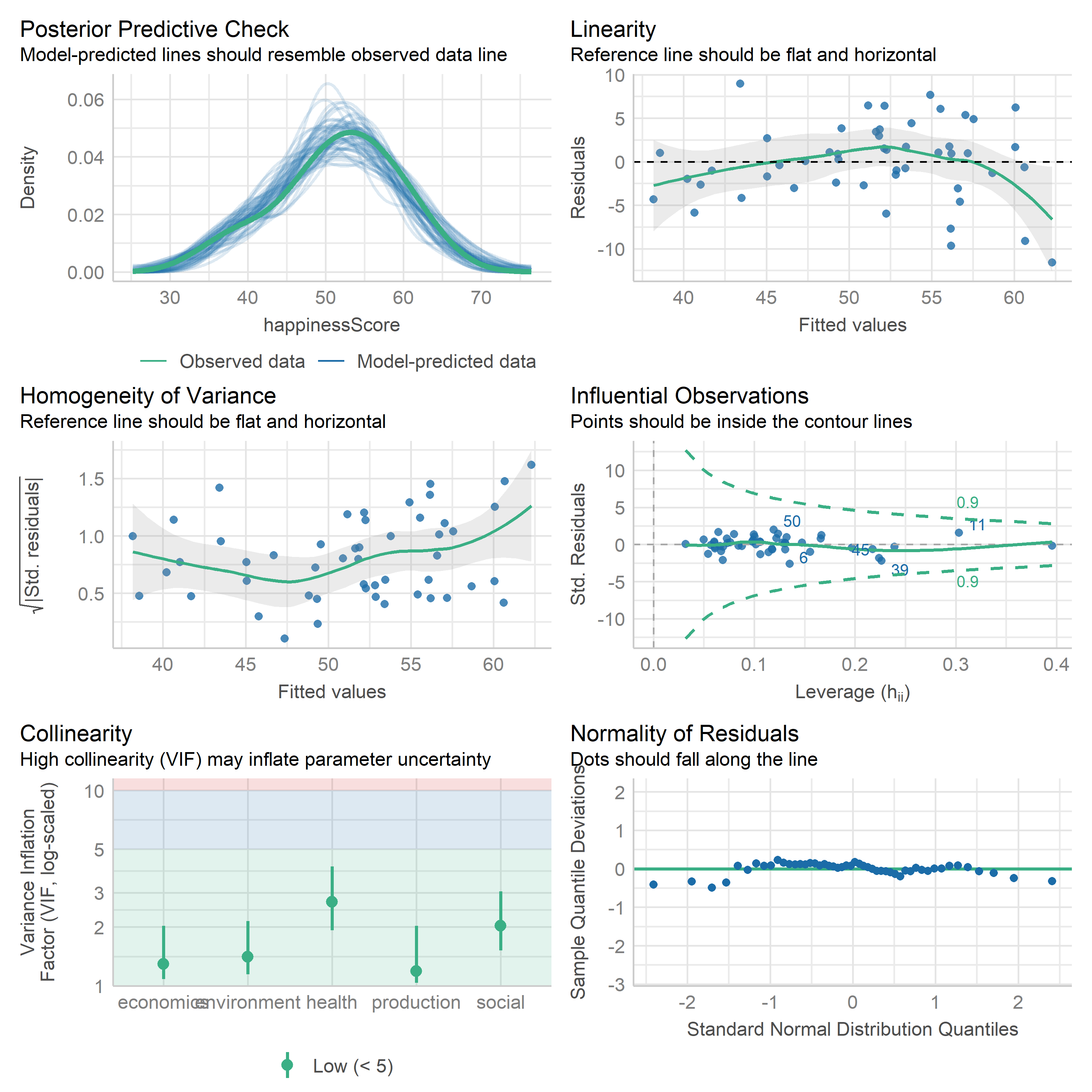
check_model(lm1)
Code
lmtest::bptest(lm1)
    studentized Breusch-Pagan test

data:  lm1
BP = 12.068, df = 5, p-value = 0.03387
2.2 Life Expectancy
Code
lm2 <-lm( lifeExpectancy ~ economics + environment + health + production + social,data = dat)
Dependent variable:
Life Expectancy
Dimensions Only
With GDP per Capita
GDP and Pop. Weights
(1)
(2)
(3)
Constant
71.837*** (70.057, 73.618)
69.820*** (67.760, 71.881)
67.969*** (65.677, 70.260)
economics
2.385 (-1.688, 6.457)
3.416 (-0.360, 7.191)
2.618 (-1.533, 6.769)
environment
-7.892*** (-11.387, -4.397)
-6.921*** (-10.170, -3.671)
-6.209** (-10.022, -2.396)
health
19.661*** (15.473, 23.849)
15.990*** (11.525, 20.455)
8.808** (3.463, 14.152)
production
2.012 (-0.601, 4.626)
1.301 (-1.127, 3.729)
1.689 (-0.060, 3.439)
social
-2.153 (-6.240, 1.934)
-1.639 (-5.386, 2.107)
2.588 (-1.390, 6.566)
gdp_per_cap
0.037** (0.014, 0.060)
0.074*** (0.049, 0.100)
WLS
No
No
Yes
Robust
No
No
No
Observations
50
50
50
R2
0.805
0.841
0.837
Adjusted R2
0.783
0.819
0.814
Residual Std. Error
0.957 (df = 44)
0.874 (df = 43)
2,099.744 (df = 43)
F Statistic
36.380*** (df = 5; 44)
37.979*** (df = 6; 43)
36.684*** (df = 6; 43)
Note:
⋆p<0.05; ⋆⋆p<0.01; ⋆⋆⋆p<0.001
Code
check_model(lm2)
Code
lmtest::bptest(lm2)
    studentized Breusch-Pagan test

data:  lm2
BP = 4.9045, df = 5, p-value = 0.4276
Code
life_exp_vcov <-vcovHC(lm2, type ='HC3')
% Table created by stargazer v.5.2.3 by Marek Hlavac, Social Policy Institute. E-mail: marek.hlavac at gmail.com % Date and time: Wed, Mar 19, 2025 - 1:50:44 PM
2.3 Food Environment Index
Code
lm3 <-lm( foodEnvironmentIndex ~ economics + environment + health + production + social,data = dat)
Dependent variable:
Food Environment Index
Dimensions Only
With GDP per Capita
GDP and Pop. Weights
(1)
(2)
(3)
Constant
3.180*** (1.905, 4.455)
2.498** (0.898, 4.098)
1.633 (0.004, 3.262)
economics
0.058 (-2.859, 2.974)
0.406 (-2.526, 3.339)
3.630* (0.678, 6.581)
environment
-0.979 (-3.482, 1.524)
-0.651 (-3.175, 1.873)
-0.450 (-3.161, 2.261)
health
12.208*** (9.208, 15.207)
10.967*** (7.498, 14.435)
10.203*** (6.403, 14.003)
production
-0.016 (-1.888, 1.855)
-0.257 (-2.143, 1.629)
-0.512 (-1.756, 0.732)
social
-1.060 (-3.987, 1.867)
-0.886 (-3.796, 2.024)
-0.870 (-3.698, 1.959)
gdp_per_cap
0.012 (-0.005, 0.030)
0.016 (-0.003, 0.034)
WLS
No
No
Yes
Robust
No
No
No
Observations
50
50
50
R2
0.769
0.779
0.810
Adjusted R2
0.743
0.748
0.784
Residual Std. Error
0.686 (df = 44)
0.679 (df = 43)
1,492.885 (df = 43)
F Statistic
29.359*** (df = 5; 44)
25.247*** (df = 6; 43)
30.644*** (df = 6; 43)
Note:
⋆p<0.05; ⋆⋆p<0.01; ⋆⋆⋆p<0.001
Code
bptest(lm3)
    studentized Breusch-Pagan test

data:  lm3
BP = 13.607, df = 5, p-value = 0.01831
Code
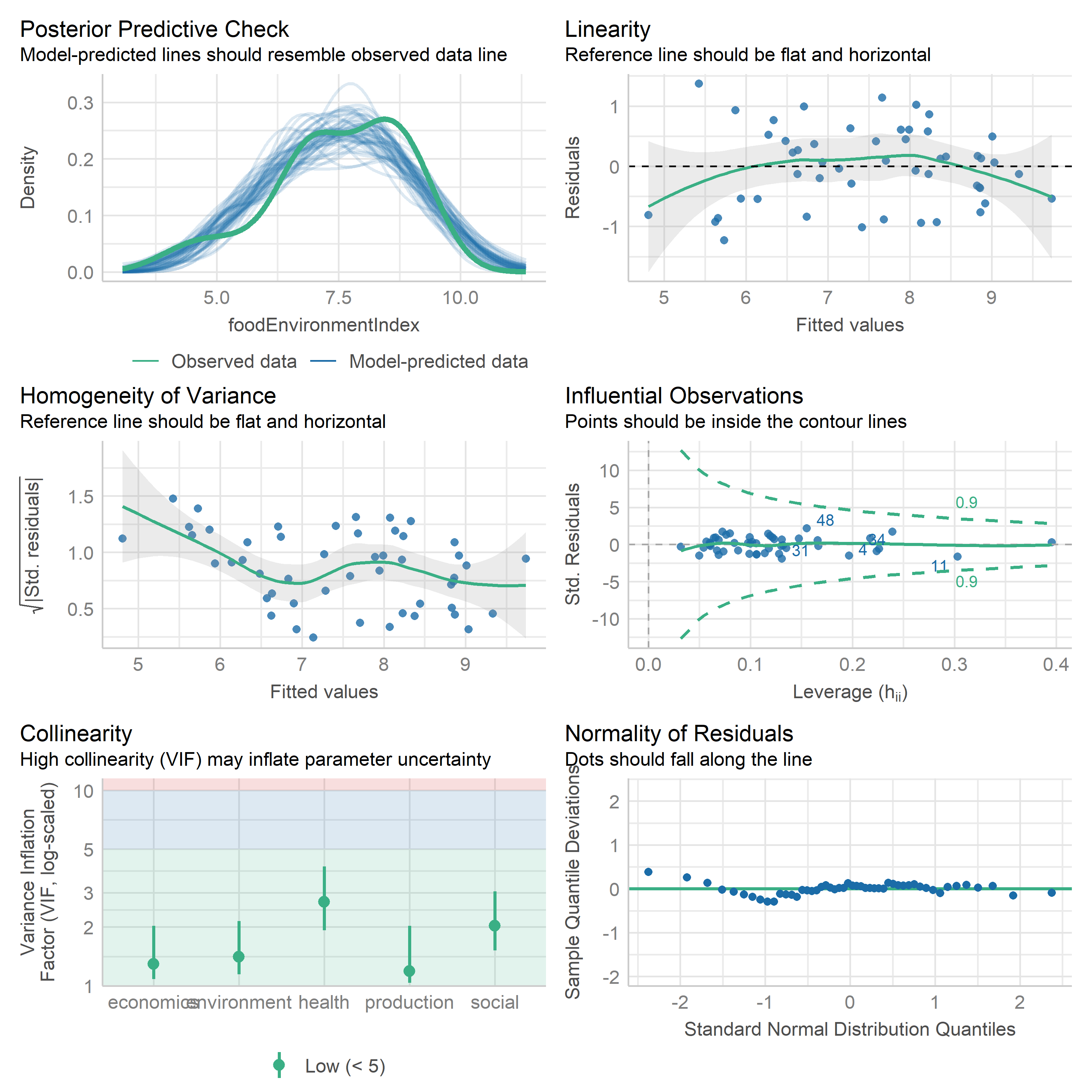
check_model(lm3)
The Food Environment Index Regression does not show heteroskedasticity, but may well have some non-linear relationships given the residual plots. Health and economics are significant predictors, with a pretty healthy \(R^2\).
Let’s try this one again with a random forest instead of linear model:
Code
# Get a version of dat without irrelevant variablesdat_ml <- dat %>%select( economics, environment, health, production, social, foodEnvironmentIndex, gdp_per_cap )# Split data 60/40set.seed(42)indices <-createDataPartition(dat_ml$foodEnvironmentIndex, p =0.60, list =FALSE)training_data <- dat_ml[indices, ]testing_data <- dat_ml[-indices,]my_folds <-createFolds(training_data$foodEnvironmentIndex, k =5, list =TRUE)# Controlmy_control <-trainControl(method ='cv',number =5,verboseIter =TRUE,index = my_folds)# Check for zero variance or near zero variance indicatorsnearZeroVar(dat, names =TRUE, saveMetrics =TRUE)# All clear# Also let's start a list with other results for preso# hyperparameters, etcml_out <-list()
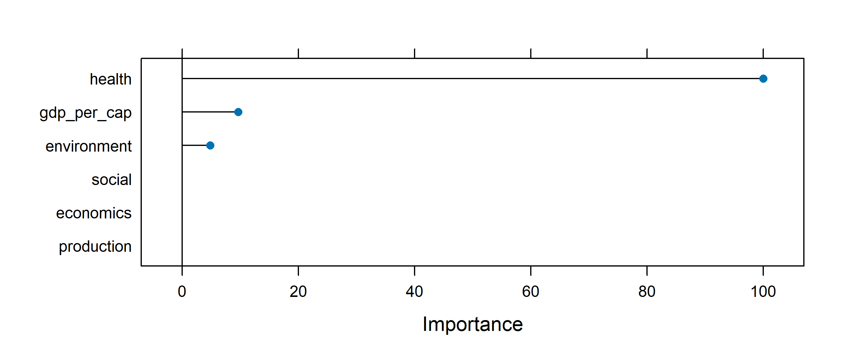
2.3.1 GLMnet
Code
set.seed(42)food_env_glmnet <-train( foodEnvironmentIndex ~ economics + environment + health + production + social + gdp_per_cap,data = training_data, tuneGrid =expand.grid(alpha =seq(0.1, 1, length =5),lambda =seq(0.0001, 0.1, length =100) ),method ="glmnet",trControl = my_control,preProcess =c('zv', 'center', 'scale'))get_str(food_env_glmnet)# Pull out best tuneml_out$glmnet_best_tune <- food_env_glmnet$bestTune
Code
importance <-varImp(food_env_glmnet, scale =TRUE)# Save for preso saveRDS(importance, 'preso/plots/val3_food_env_glmnet_importance.rds')#pred <-predict(food_env_glmnet, testing_data)ml_out$glmnet_performance <-postResample(pred = pred, obs = testing_data$foodEnvironmentIndex) %>%round(3)# ml_out$glmnet_performanceml_out$glmnet_imp_plot <- importance %>%ggplot(aes(x = Overall, y =rownames(.))) +geom_col(color ='royalblue',fill ='lightblue' ) +theme_classic() plot(importance)
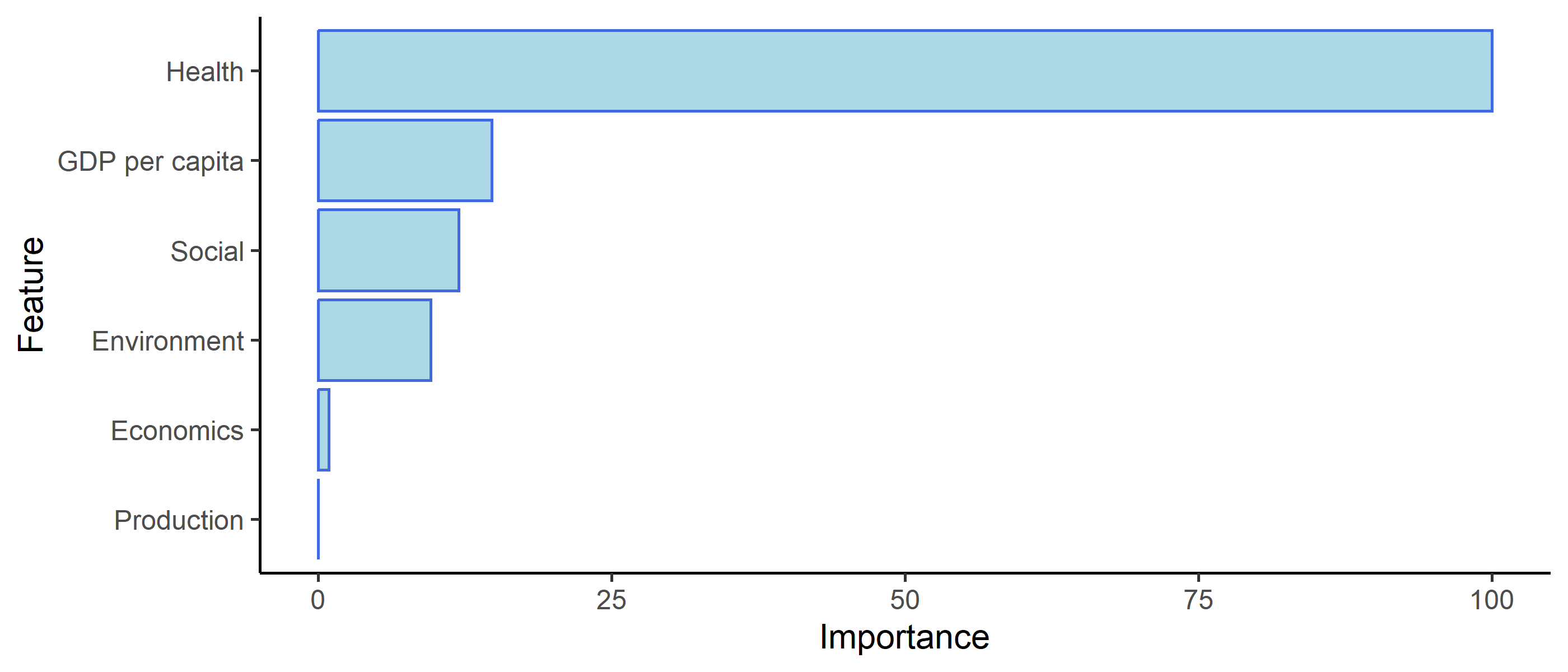
2.3.2 Random Forest
Code
set.seed(42)food_env_rf <-train( foodEnvironmentIndex ~ production + social + health + economics + environment + gdp_per_cap,data = training_data, tuneLength =7,method ="ranger",trControl = my_control,importance ='impurity')get_str(food_env_rf)# Pull out best tuneml_out$rf_best_tune <- food_env_rf$bestTune
OOB prediction error (MSE): 0.6360507
Code
importance <-varImp(food_env_rf, scale =TRUE)# Save for presosaveRDS(importance, 'preso/plots/val3_rf_importance.rds')# Get RMSEA and stuffpred <-predict(food_env_rf, testing_data)ml_out$rf_performance <-postResample(pred = pred, obs = testing_data$foodEnvironmentIndex) %>%round(3)# ml_out$rf_performanceimp <- importance$importance %>%as.data.frame() %>% tibble::rownames_to_column() %>%setNames(c('Feature', 'Importance')) %>%mutate(Importance =round(Importance, 2)) %>%arrange(desc(Importance)) %>%mutate(Feature = Feature %>%str_to_title() %>%str_replace('Gdp_per_cap', 'GDP per capita') )ml_out$rf_imp_plot <- imp %>%ggplot(aes(x = Importance, y =reorder(Feature, Importance),text =paste0('<b>Variable:</b> ', Feature, '\n','<b>Importance:</b> ', Importance ) )) +geom_col(color ='royalblue',fill ='lightblue', ) +theme_classic() +labs(x ='Importance',y ='Feature' )# Save all results for presosaveRDS(ml_out, 'preso/data/ml_out.rds')# Show plotml_out$rf_imp_plot
2.4 Happiness Score
Code
lm4 <-lm( happinessScore ~ economics + environment + health + production + social,data = dat)
Dependent variable:
Happiness Index
Dimensions Only
With GDP per Capita
GDP and Pop. Weights
(1)
(2)
(3)
Constant
32.347*** (23.503, 41.191)
25.028*** (14.265, 35.791)
25.015*** (14.267, 35.763)
economics
23.038* (2.804, 43.271)
26.779* (7.056, 46.502)
24.625* (5.152, 44.098)
environment
-34.924*** (-52.287, -17.561)
-31.401*** (-48.376, -14.425)
-26.400** (-44.286, -8.513)
health
57.152*** (36.346, 77.959)
43.831*** (20.505, 67.156)
40.807** (15.736, 65.878)
production
13.655* (0.671, 26.638)
11.074 (-1.610, 23.759)
6.970 (-1.238, 15.178)
social
-2.149 (-22.454, 18.156)
-0.286 (-19.858, 19.287)
3.405 (-15.257, 22.067)
gdp_per_cap
0.134* (0.013, 0.254)
0.130* (0.010, 0.250)
WLS
No
No
Yes
Robust
No
No
No
Observations
50
50
50
R2
0.655
0.689
0.717
Adjusted R2
0.616
0.646
0.677
Residual Std. Error
4.757 (df = 44)
4.568 (df = 43)
9,849.609 (df = 43)
F Statistic
16.709*** (df = 5; 44)
15.882*** (df = 6; 43)
18.125*** (df = 6; 43)
Note:
⋆p<0.05; ⋆⋆p<0.01; ⋆⋆⋆p<0.001
Code
check_model(lm4)
3 PCA
Let’s use PCA to see how our indicators are associated with a set of orthogonal components. Ideally, we might like to see that each indicator is associated strongly with a single component (simple structure) that corresponds to the dimension.
3.1 Component Extraction
First we determine how many components to extract. This is a bit subjective, so we will use a few methods.
Code
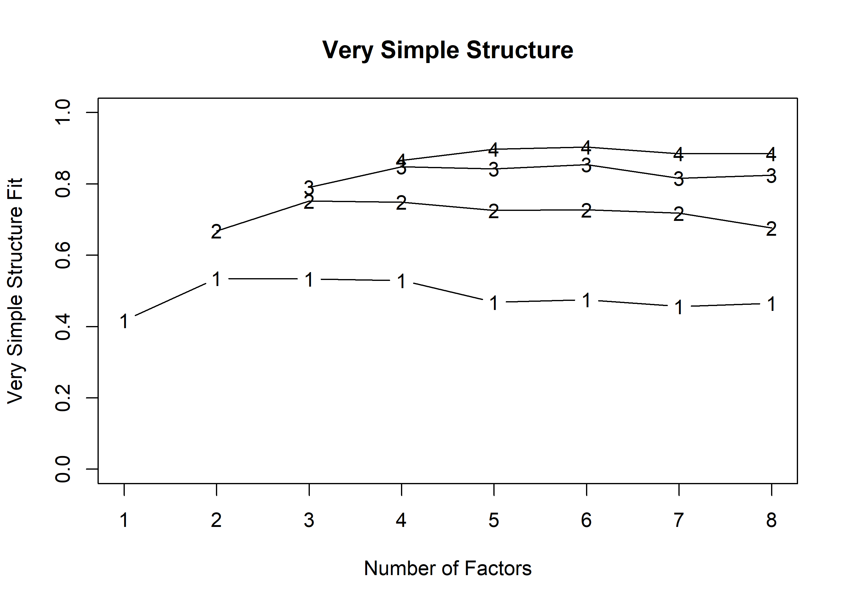
raw_minmax_geo <-readRDS('data/raw_minmax_geo.rds')framework <-readRDS('data/filtered_frame.rds')# Filter down to just indicators for PCApca_dat <- raw_minmax_geo %>%select(starts_with('indic')) %>%setNames(c(str_remove(names(.), 'indic_'))) %>%as.data.frame()# get_str(pca_dat)# Explore how many factors to extractVSS(pca_dat, n =8, fm ='pc', rotate ='Promax')
Very Simple Structure
Call: vss(x = x, n = n, rotate = rotate, diagonal = diagonal, fm = fm,
    n.obs = n.obs, plot = plot, title = title, use = use, cor = cor)
VSS complexity 1 achieves a maximimum of 0.53  with  2  factors
VSS complexity 2 achieves a maximimum of 0.75  with  3  factors

The Velicer MAP achieves a minimum of 0.04  with  6  factors
BIC achieves a minimum of Inf with factors
Sample Size adjusted BIC achieves a minimum of  Inf  with    factors

Statistics by number of factors
  vss1 vss2   map dof chisq prob sqresid  fit RMSEA BIC SABIC complex eChisq
1 0.42 0.00 0.069   0    NA   NA    85.4 0.42    NA  NA    NA      NA     NA
2 0.53 0.67 0.059   0    NA   NA    48.6 0.67    NA  NA    NA      NA     NA
3 0.53 0.75 0.055   0    NA   NA    30.7 0.79    NA  NA    NA      NA     NA
4 0.53 0.75 0.046   0    NA   NA    19.6 0.87    NA  NA    NA      NA     NA
5 0.47 0.73 0.039   0    NA   NA    13.2 0.91    NA  NA    NA      NA     NA
6 0.48 0.73 0.039   0    NA   NA    10.5 0.93    NA  NA    NA      NA     NA
7 0.46 0.72 0.041   0    NA   NA     8.5 0.94    NA  NA    NA      NA     NA
8 0.47 0.68 0.040   0    NA   NA     6.5 0.96    NA  NA    NA      NA     NA
  SRMR eCRMS eBIC
1   NA    NA   NA
2   NA    NA   NA
3   NA    NA   NA
4   NA    NA   NA
5   NA    NA   NA
6   NA    NA   NA
7   NA    NA   NA
8   NA    NA   NA
Code
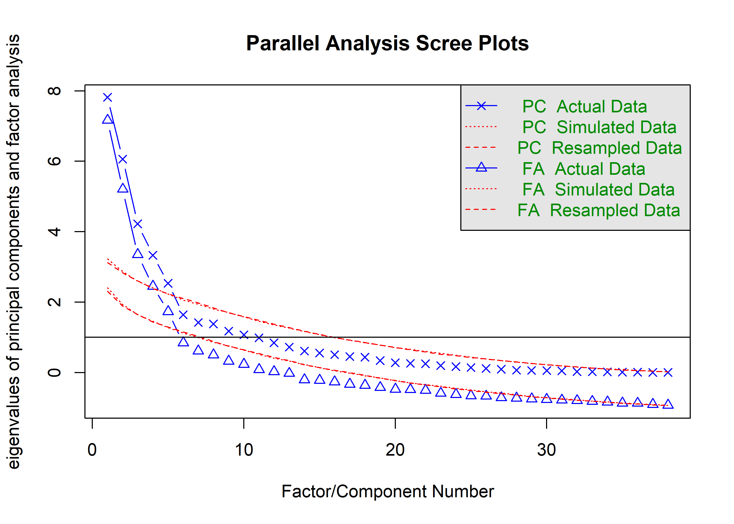
set.seed(42)fa.parallel(pca_dat, fm ='ml')
Parallel analysis suggests that the number of factors = 5 and the number of components = 5
MAP suggests 6, VSS 2 or 3, PA suggests 5. Not half bad. I think we are justified to go with 5.
Code
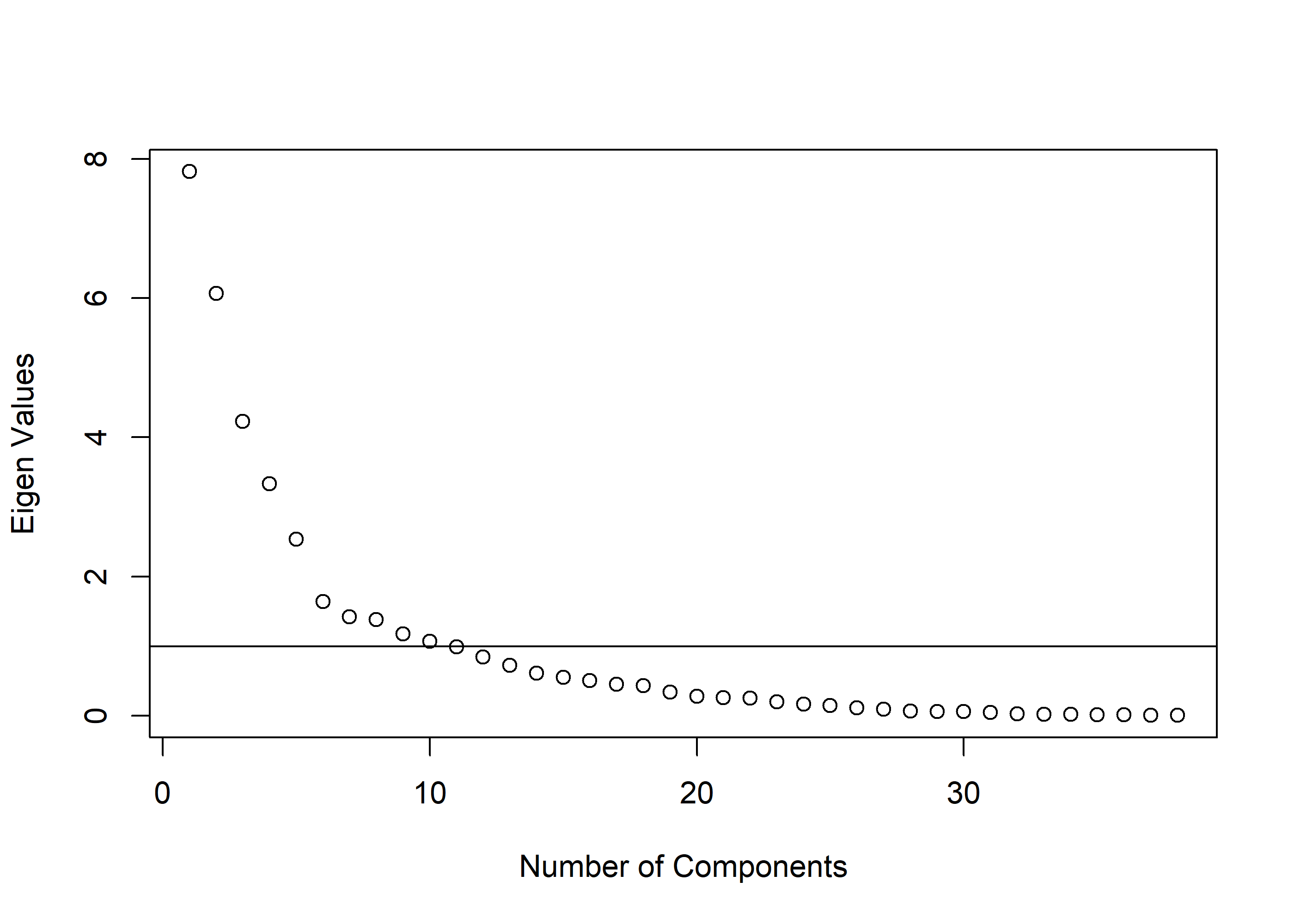
# Oblique rotations: promax, oblimin, simplimax, clusterrotations <-c('Promax','oblimin','simplimax','cluster')pca_outs <-map(rotations, ~ { pca_dat %>%# scale() %>% pca(nfactors =5, rotate = .x)}) %>%setNames(c(rotations))# Save a version of promax for preso?png(filename ='preso/plots/scree.png',width =800,height =600,units ='px',res =150)plot( pca_outs$simplimax$values,xlab ='Number of Components',ylab ='Eigen Values')abline(h =1)dev.off()
png
  2
Code
# Now actually show it plot( pca_outs$simplimax$values,xlab ='Number of Components',ylab ='Eigen Values')abline(h =1)
The scree plot makes a reasonably convincing case for 6 components, as the slope falls off substantially after the fifth.
Note that we are using the promax rotation here as it seemed most interpretable, but we have created and saved all the other available oblique rotations as well.
It looks like our economics indicators are quite scattered, but the environment indicators mostly stick to components 3 and 4. Health is quite well centered on component 3, although the “physical health tbd” indicator has meaningful loadings on three components. Production and social are rather scattered, and it is also noteworthy that participatory governance is associated with three components as well.