First trying linear models with time as independent variable. Normalizing dataset before we do anything else.
Code
get_str(datasets$dp_metrics_county)# Function to min max then scale to 0 to 100 for percent changemin_max <-function(x) { normed <- (x -min(x, na.rm =TRUE)) / (max(x, na.rm =TRUE) -min(x, na.rm =TRUE)) normed *100}vars <-unique(datasets$dp_metrics_county$variable_name)datasets$dp_metrics_county <-map(vars, ~ { datasets$dp_metrics_county %>%filter(variable_name == .x) %>%drop_na(value) %>%group_by(variable_name) %>%mutate(normed_value =min_max(value)) %>%ungroup()}) %>%list_rbind()get_str(datasets$dp_metrics_county)
1.1 Regressions
First create a weights crosswalk that links variable_names to weighting variables.
Code
weights_crosswalk <-data.frame(metric =c('GDP','GDP from agriculture','Total number of producers','Total number of operations','Population (annual)','Population (5 year)','Population (5 year, smooth)','Acres of land','Acres of water','Area under agriculture (CDL)','Number employed in agriculture','Acres operated','Acres operated, smooth','Acres of cropland ag land','Acres of woodland ag land','Acres of pasture ag land','Total farm income','Total sales from commodities' ),variable_name =c('gdp','gdpFromAg','nProducers','nOperations','populationAnnual','population5Year','population5YearSmooth','landAcres','waterAcres','cdlAgAcres','annualAvgEmplvlNAICS11','acresOperated','acresOperatedSmooth','agLandCropAcres','agLandWoodAcres','agLandPastureAcres','totalFarmIncome','totalSalesCommodities' ))weights_crosswalk# Link weight vars to the appropriate variablesweights_crosswalk <- data_paper_meta %>%select(variable_name, weighting) %>%filter(variable_name %in% datasets$dp_metrics_county$variable_name) %>%left_join(weights_crosswalk, by =join_by(weighting == metric)) %>%setNames(c('variable_name', 'weight_metric', 'weight_variable')) %>%select(-weight_metric) %>%na.omit()get_str(weights_crosswalk)weights_crosswalk
Run regressions for all time series variables where time points > 1.
Code
# Get a crosswalk to add state as a fixed effectstate_link <- fips_key %>%filter(str_length(fips) ==2, fips !='00') %>%select(fips, state_code)res <-map(datasets$series_vars, ~ {tryCatch( { df <- datasets$dp_metrics_county %>%filter(variable_name == .x) %>%mutate(value =as.numeric(value),year =as.numeric(year),state_fips =str_sub(fips, end =2) ) %>%left_join(state_link, by =join_by(state_fips == fips))# Add weighting variable weight_var <- weights_crosswalk$weight_variable[weights_crosswalk$variable_name == .x] weight_df <- datasets$dp_weightsif (!is.na(weight_var) &&length(weight_var) >0) { weight_df <- weight_df %>%filter(variable_name == weight_var) } weight_df <- weight_df %>%mutate(value =as.numeric(value), year =as.numeric(year) ) %>%rename(weight_value = value, weight_name = variable_name,weight_year = year )# get_str(weight_df)# Depending on whether weight has a year, do appropriate join# Note that we might be losing some years here if weighting var doesn't# cover the variable enoughif (all(is.na(weight_df$weight_year))) { df <- df %>%inner_join(weight_df, by =join_by(fips)) } else { df <- df %>%inner_join(weight_df, by =join_by(fips, year == weight_year)) }# Reduce to county fips only. Remove dupes df <- df %>%filter(str_length(fips) ==5) %>%distinct()# Weighted OLS model <-lm( normed_value ~ year + state_code, data = df,weights = weight_value )return(model) },error =function(e) {message(paste('Error with var', .x)) } )}) %>%setNames(c(datasets$series_vars)) %>%discard(\(x) is.null(x))get_str(res, 1)get_str(res)# Robust SEspacman::p_load(lmtest)coeftest(res[[1]])# Save immediate outputsaveRDS(res, 'data/objects/weighted_ols_outs.rds')
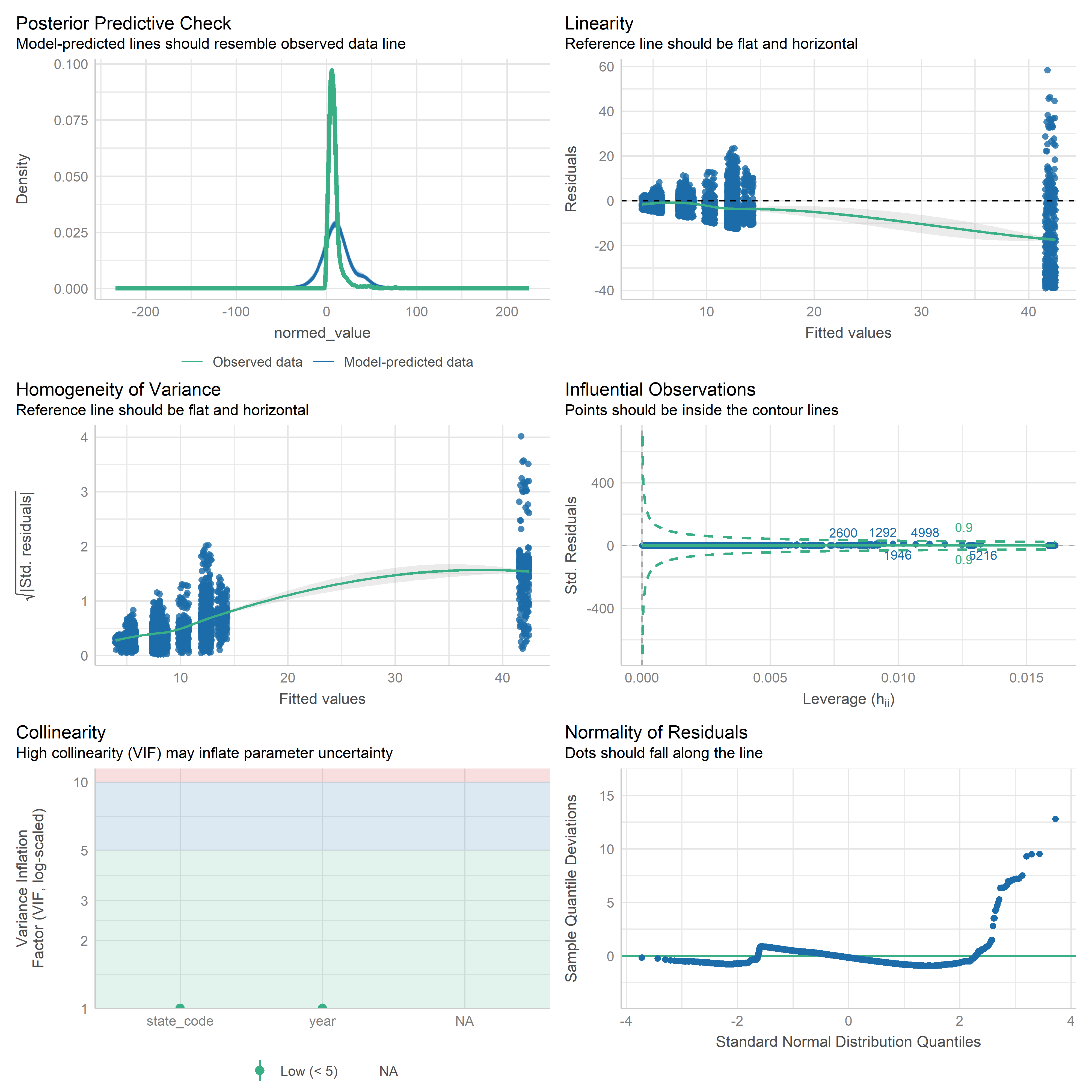
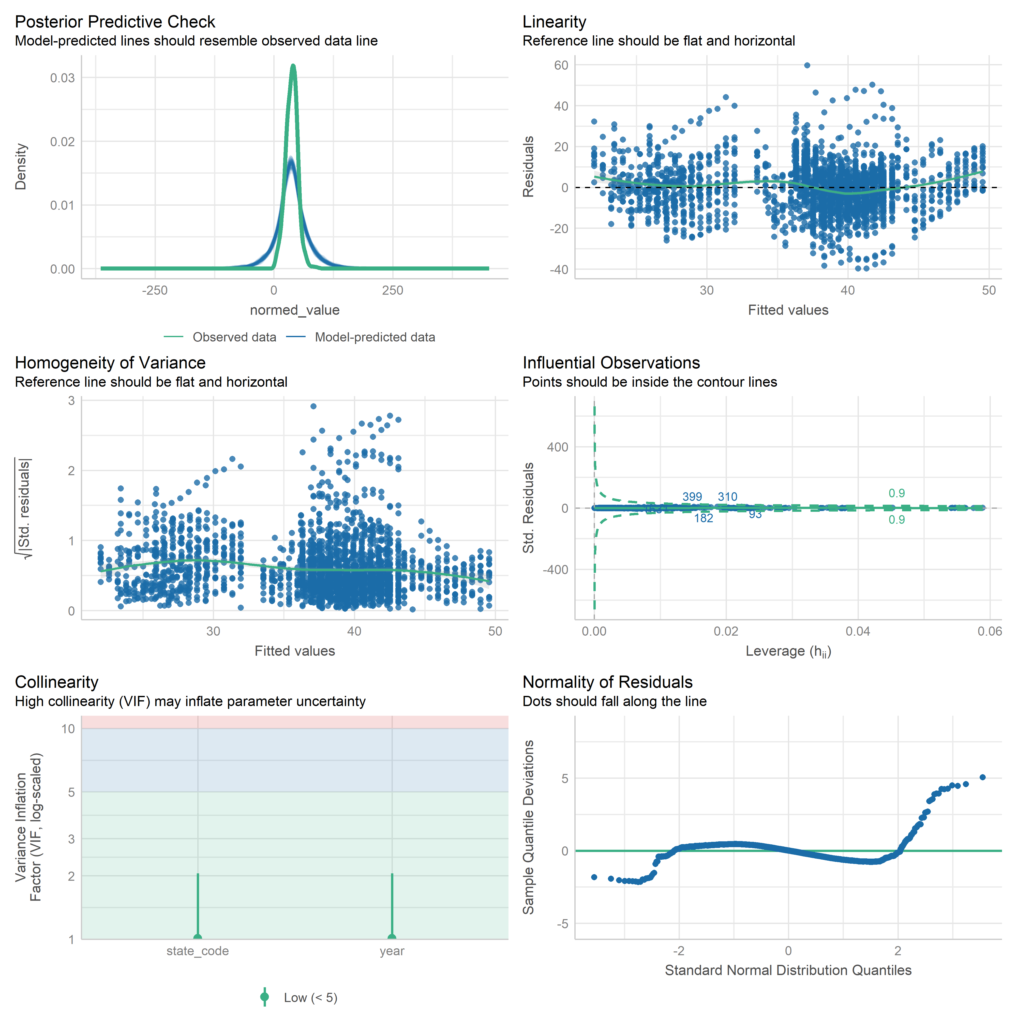
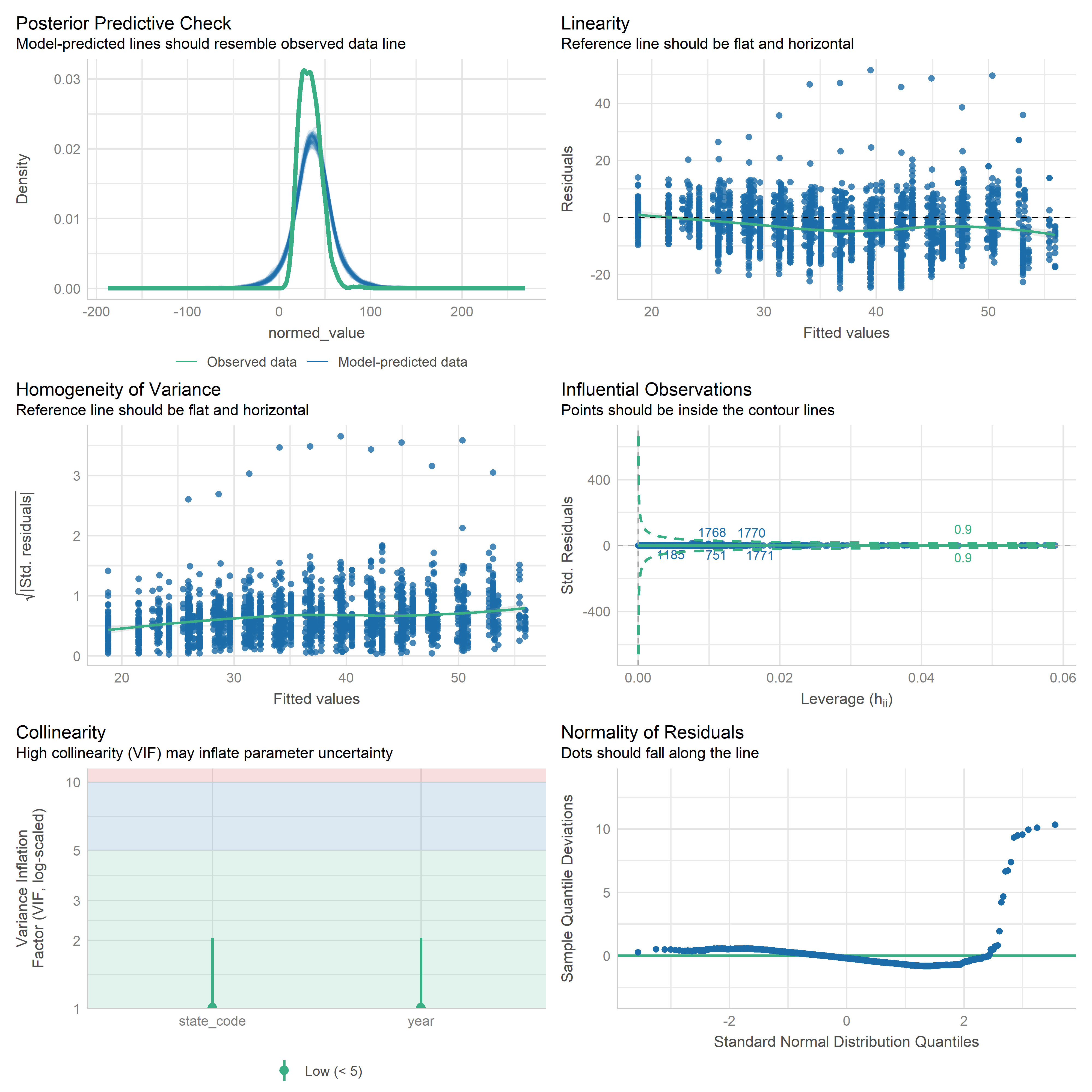
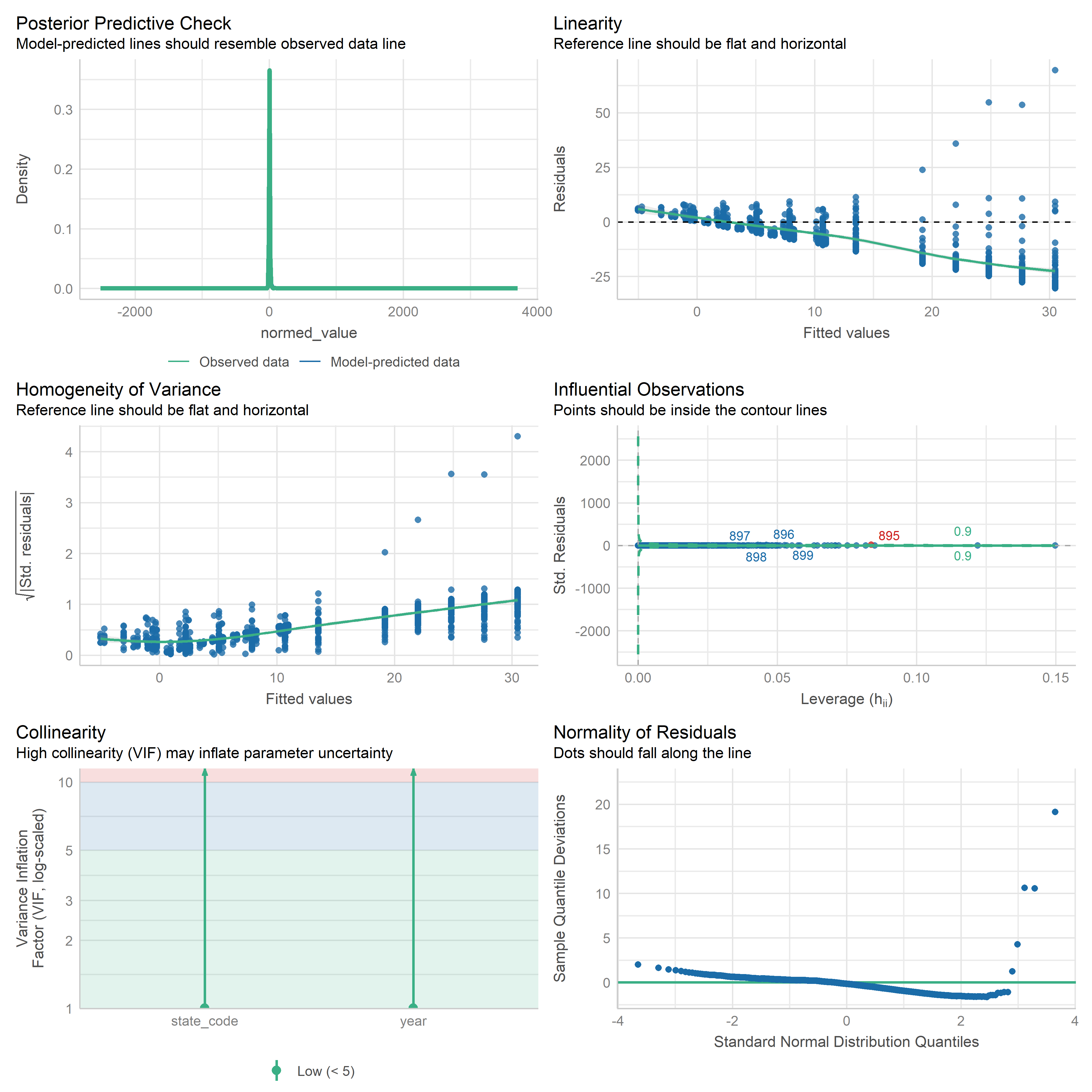
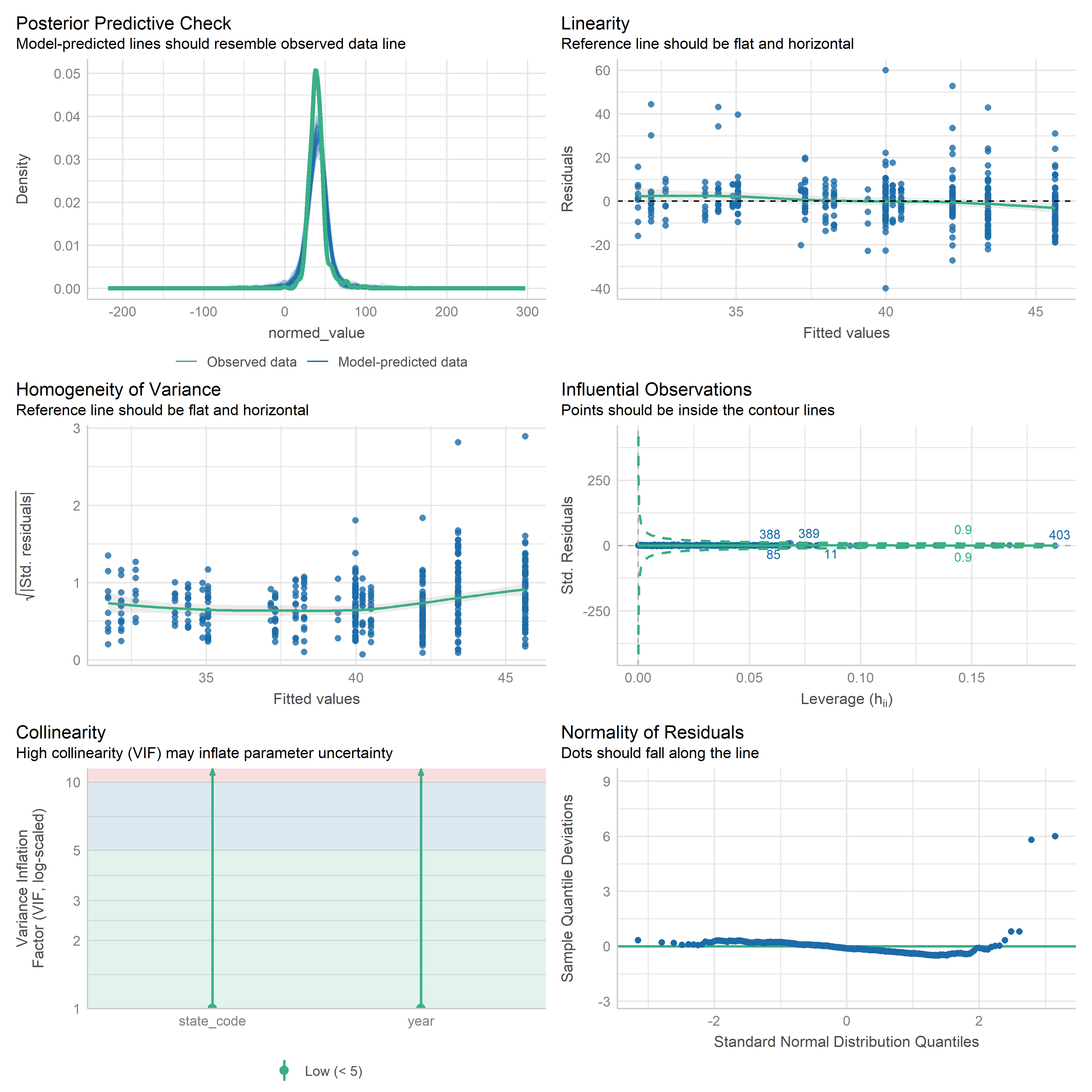
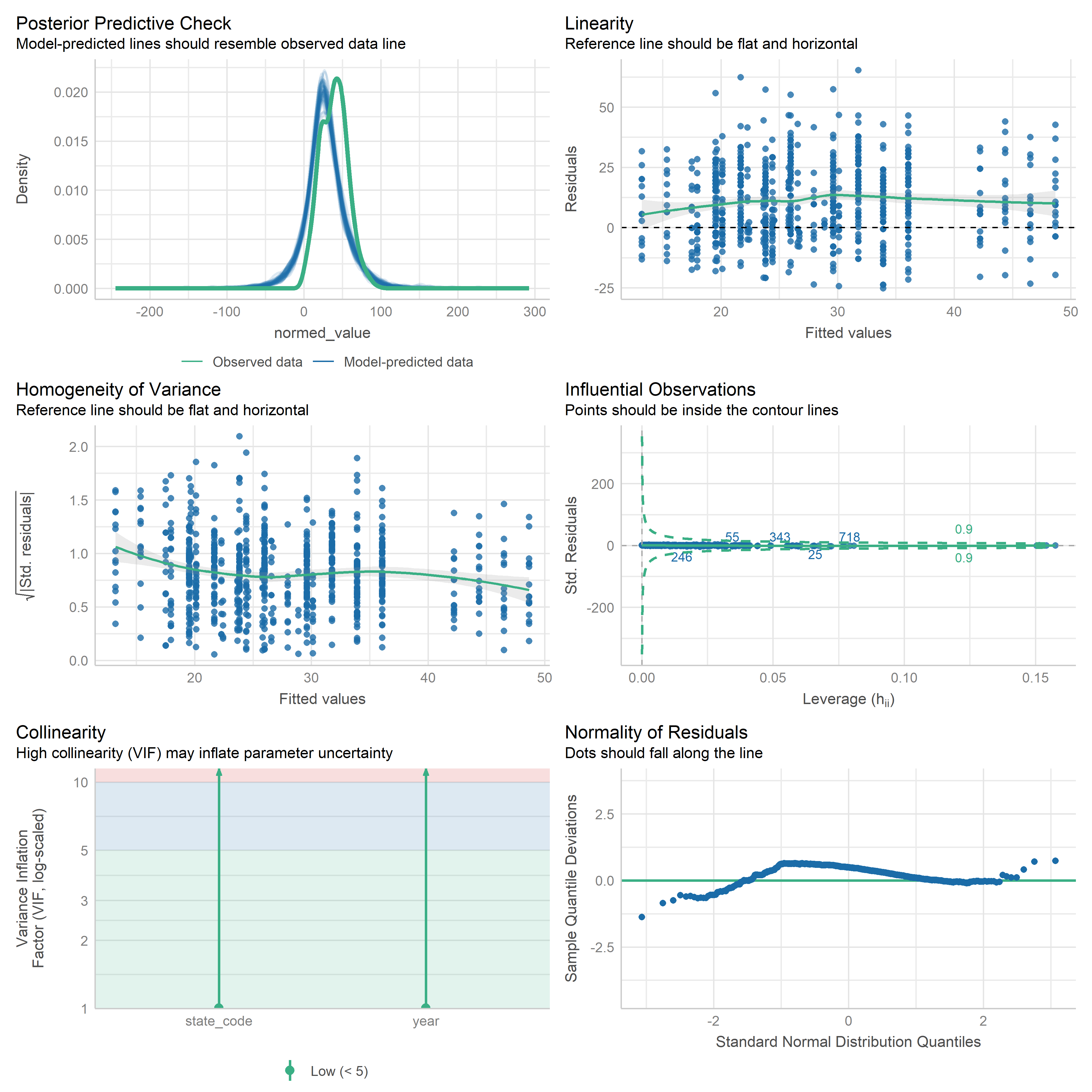
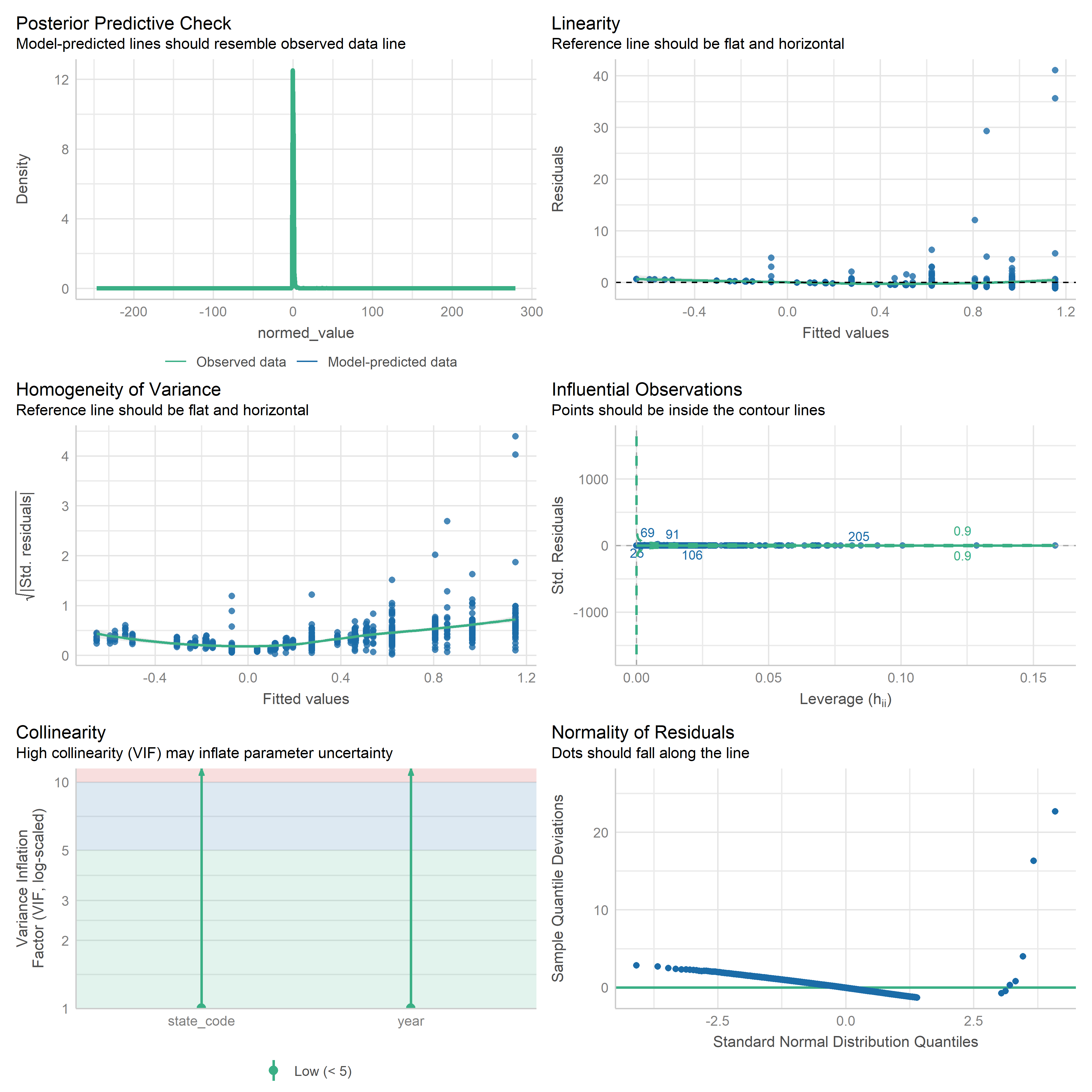
1.2 Residuals
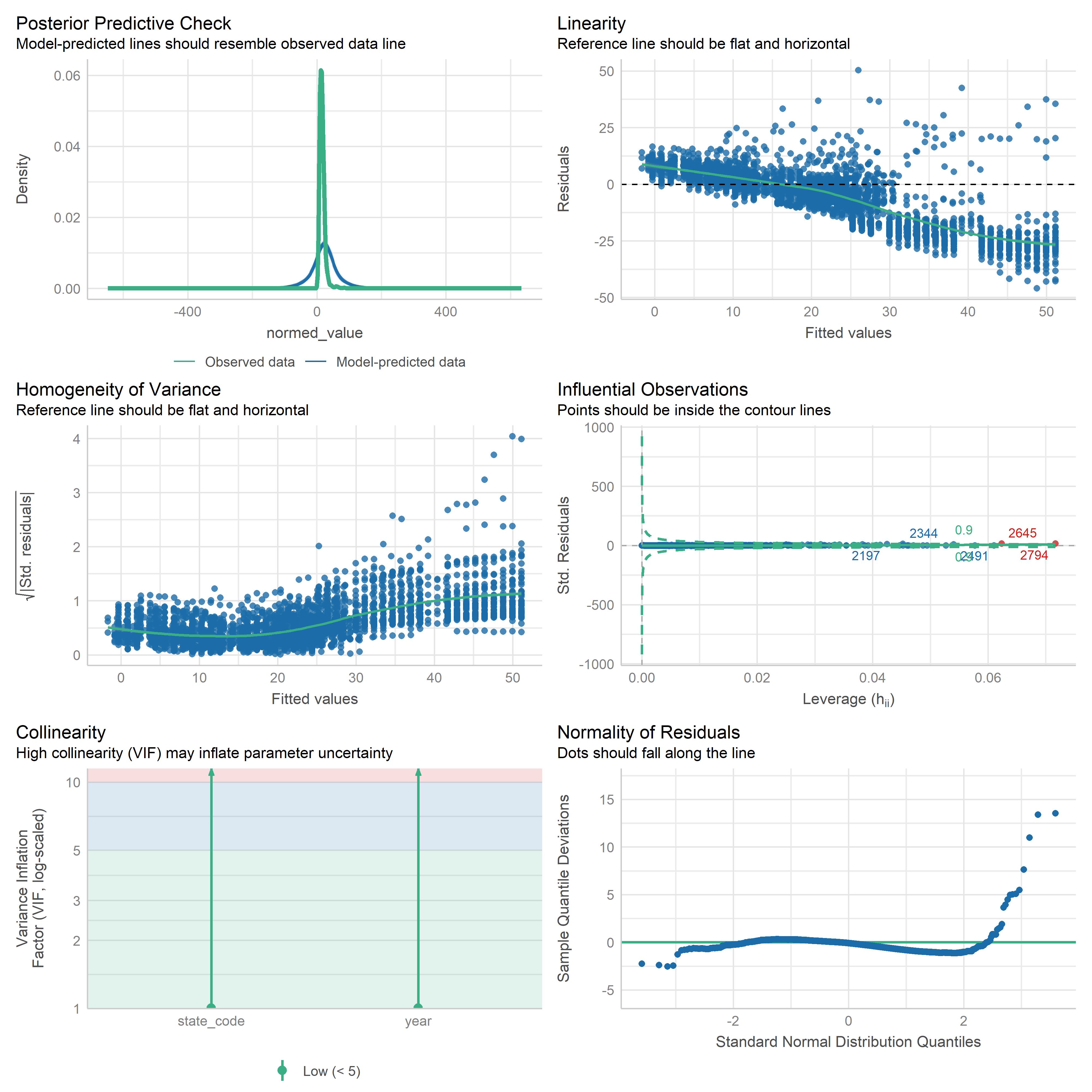
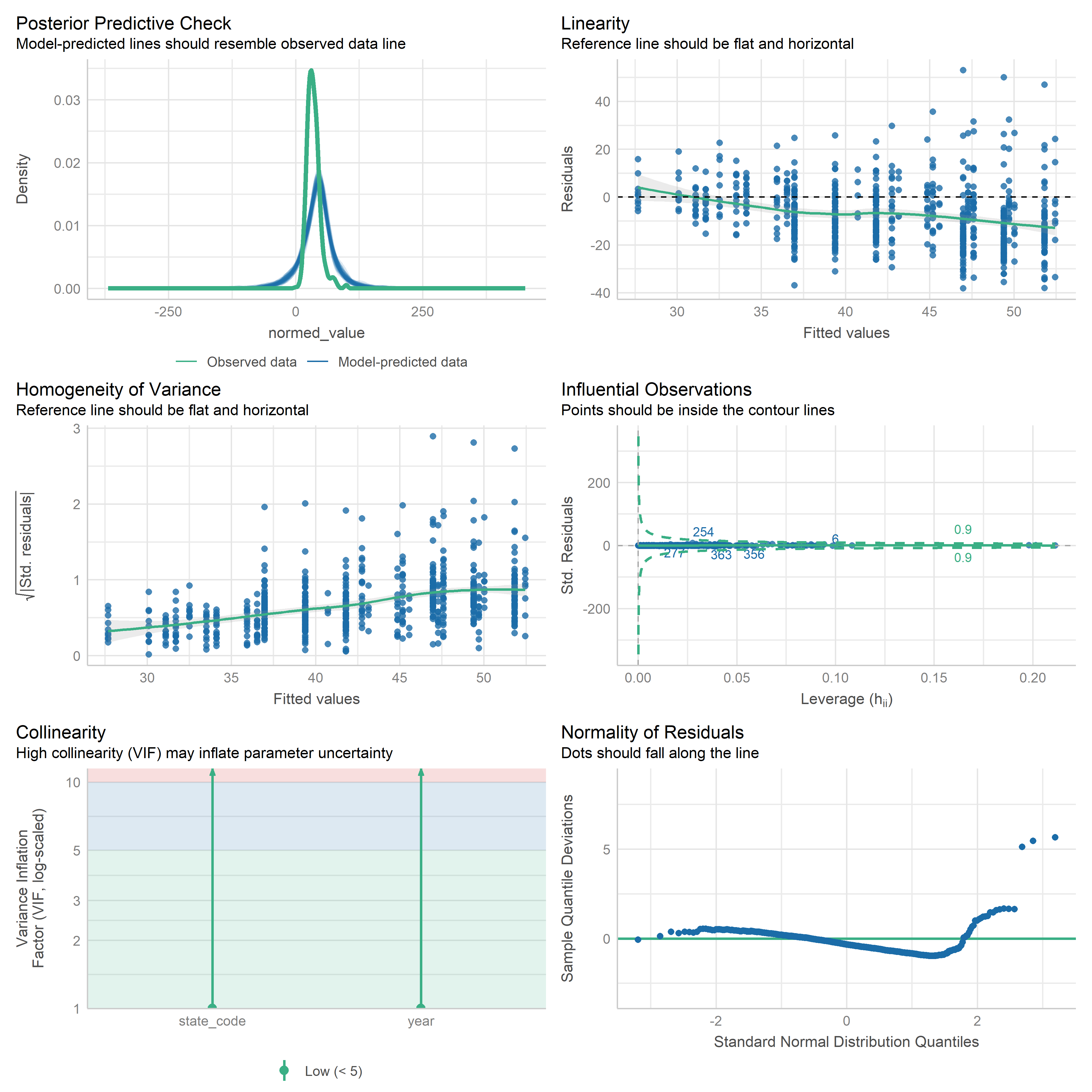
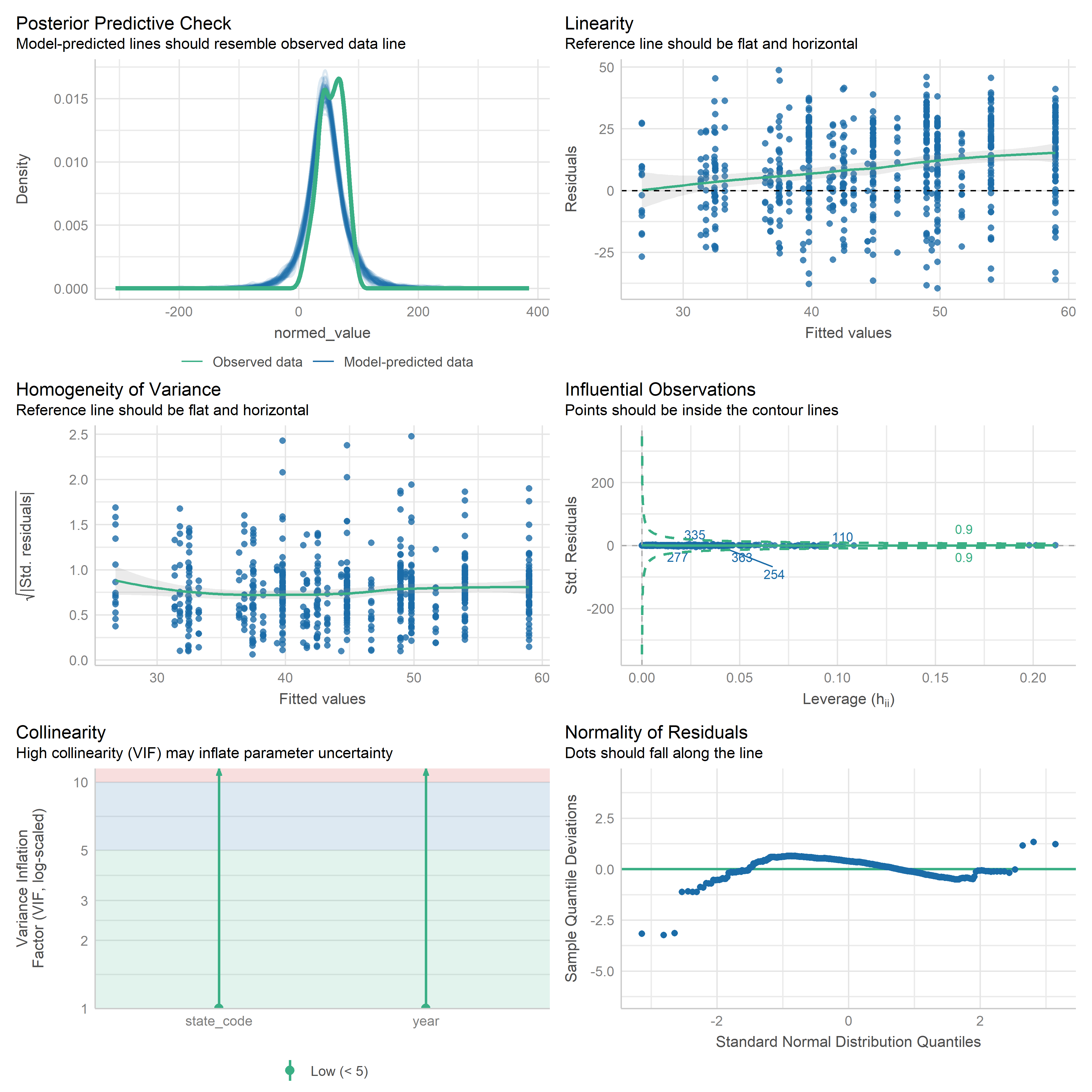
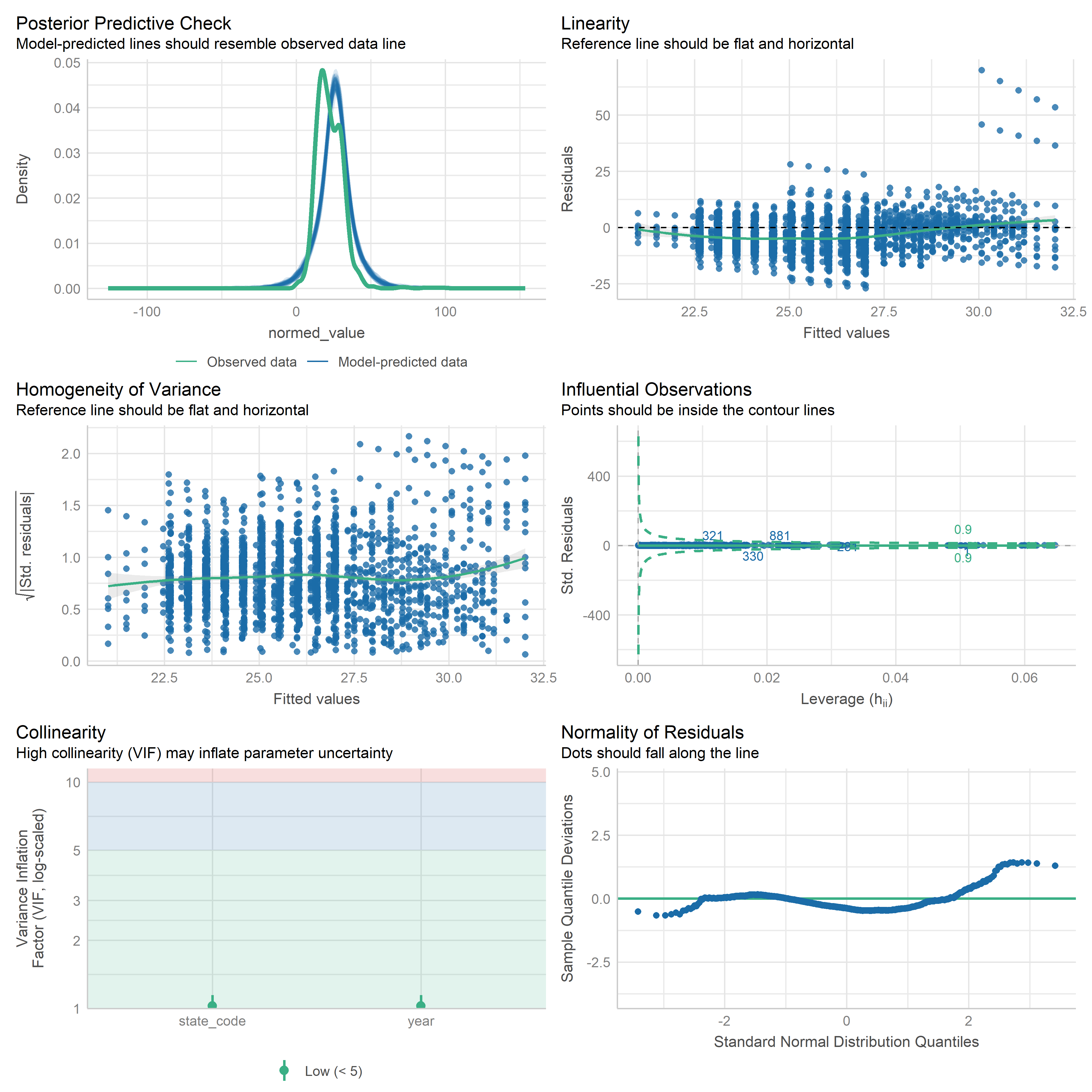
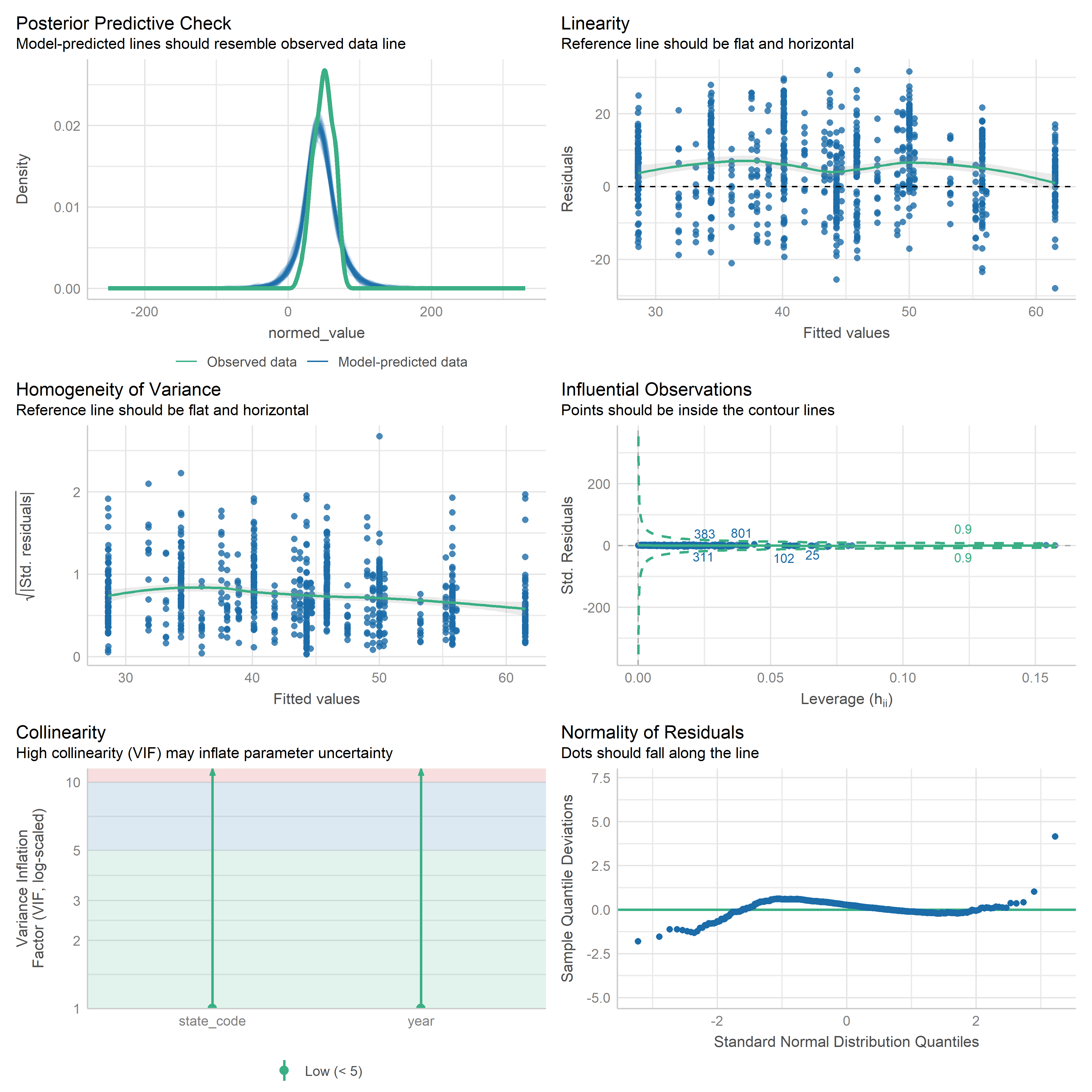
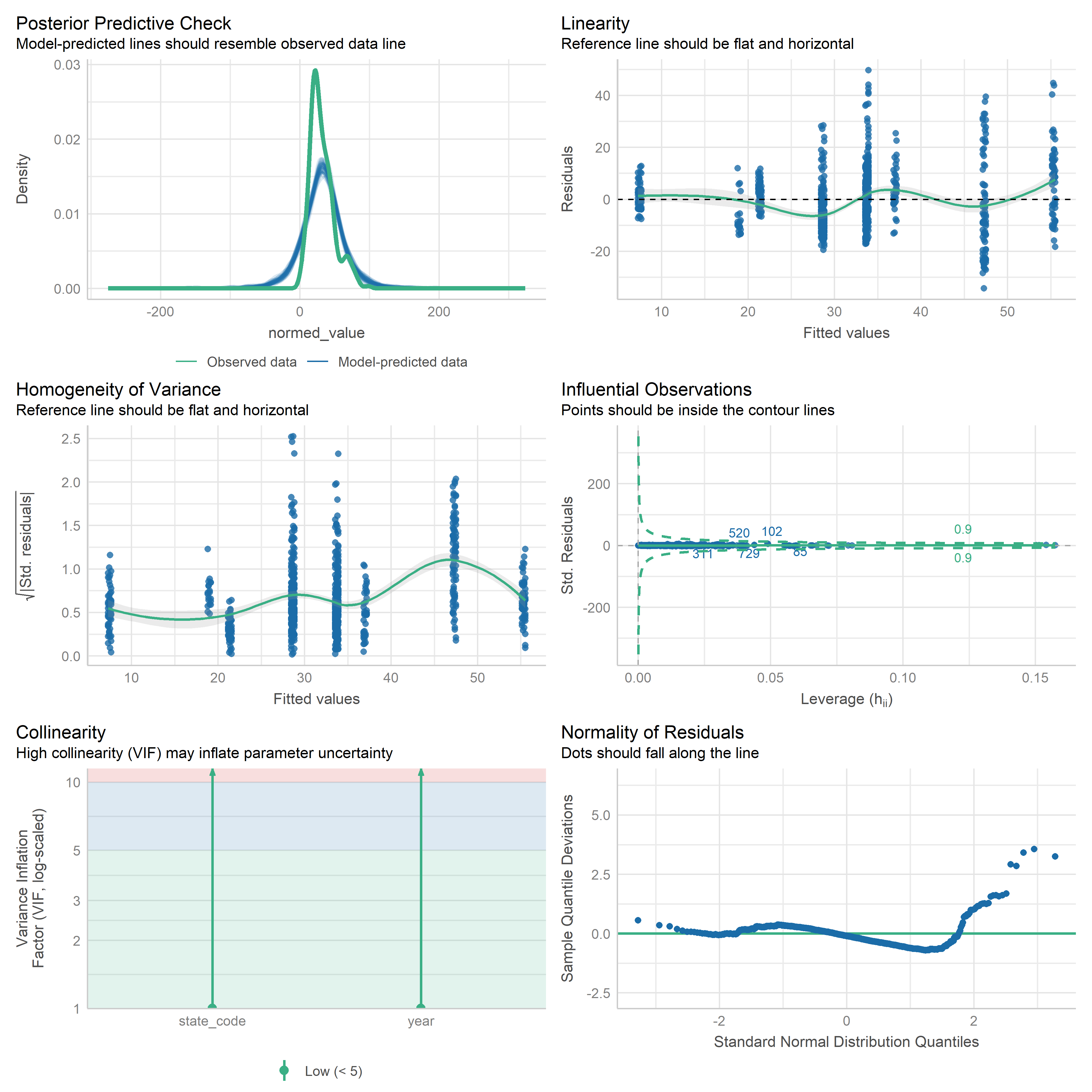
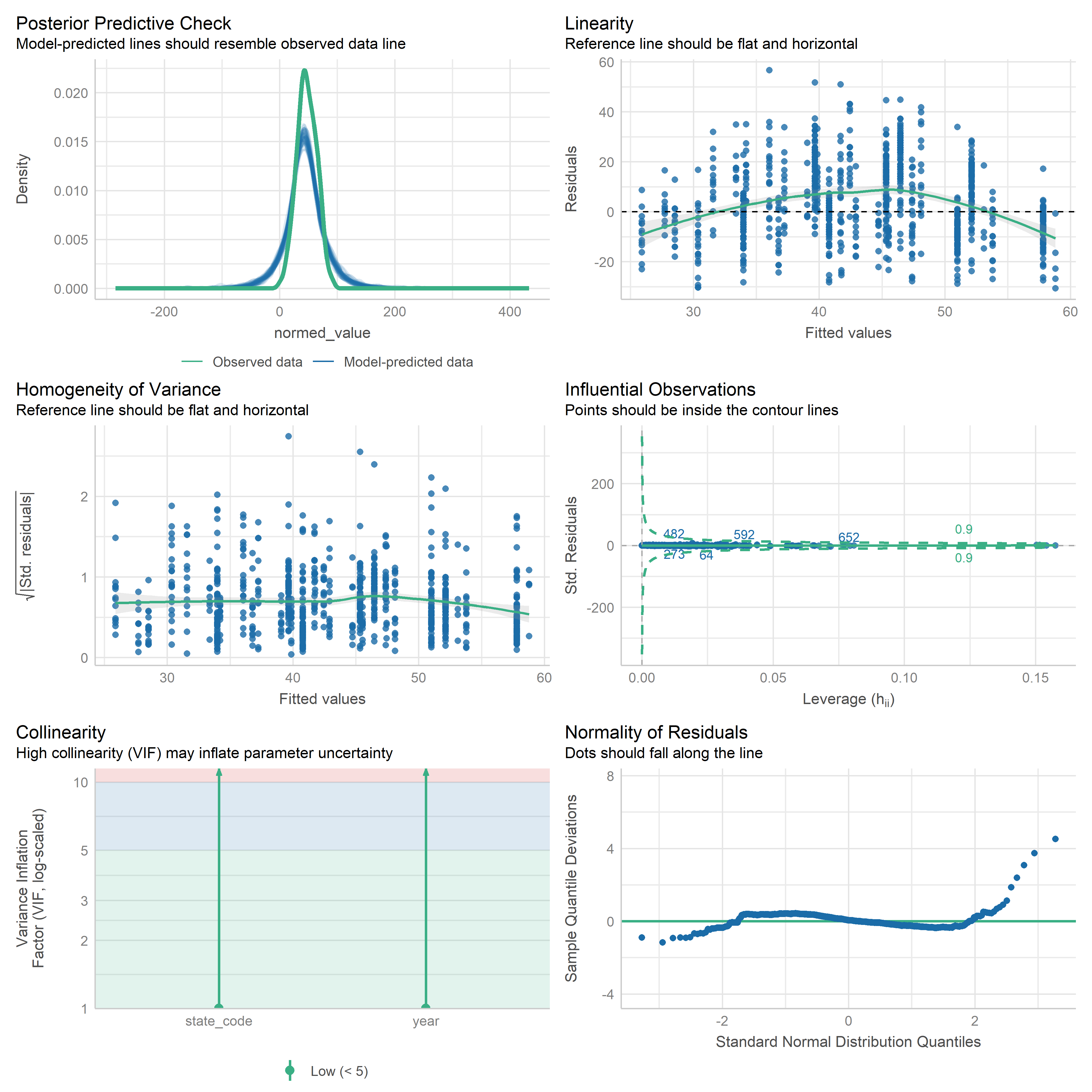
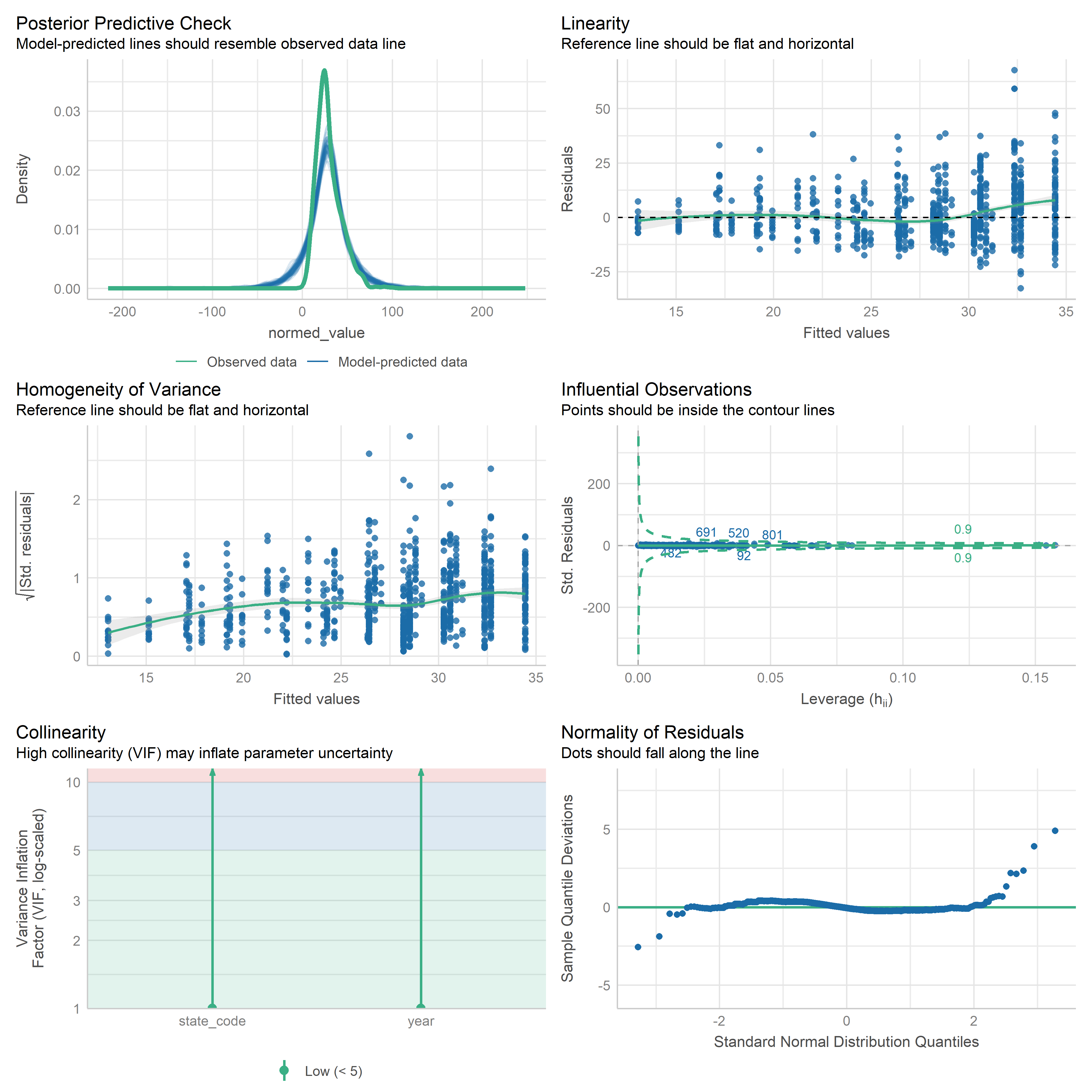
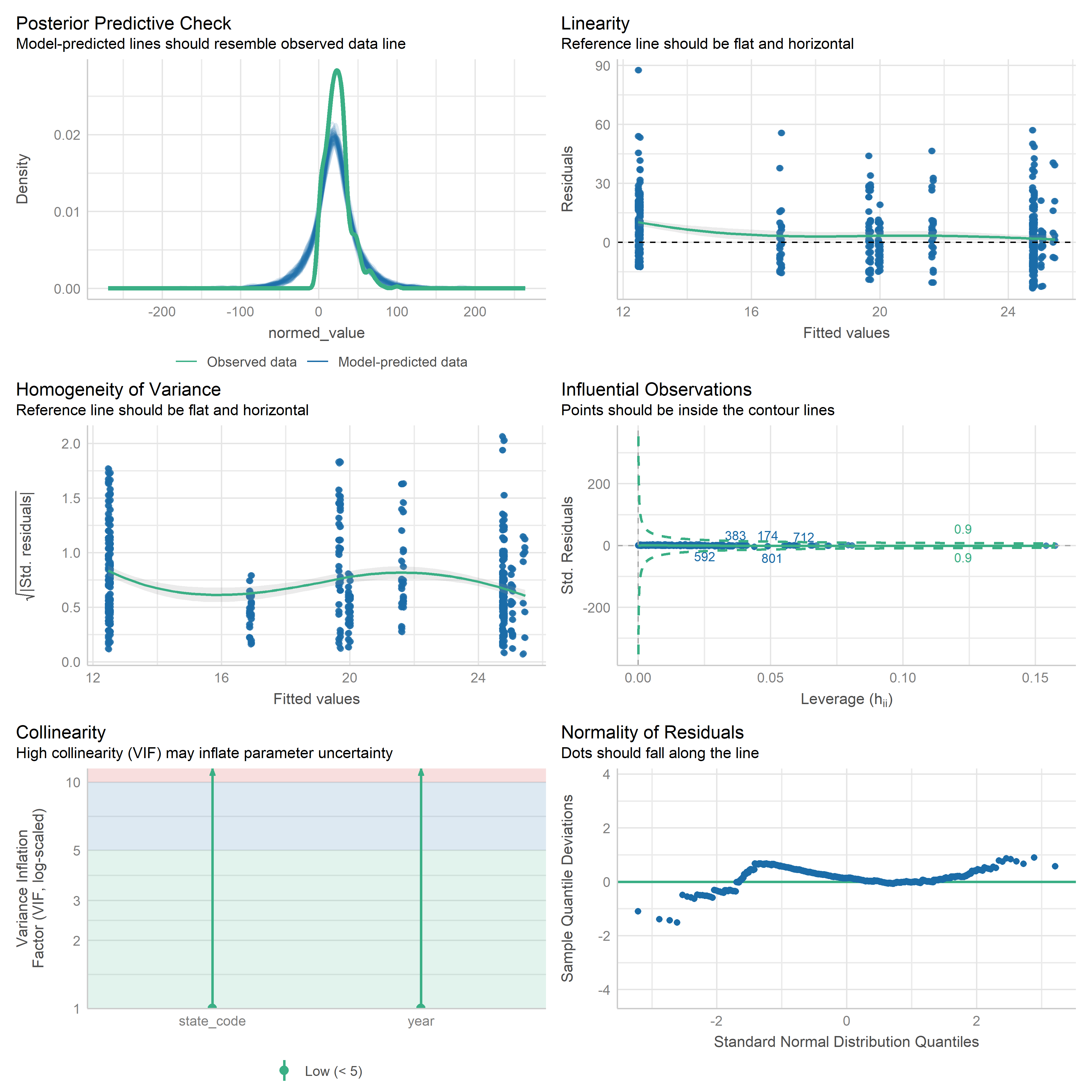
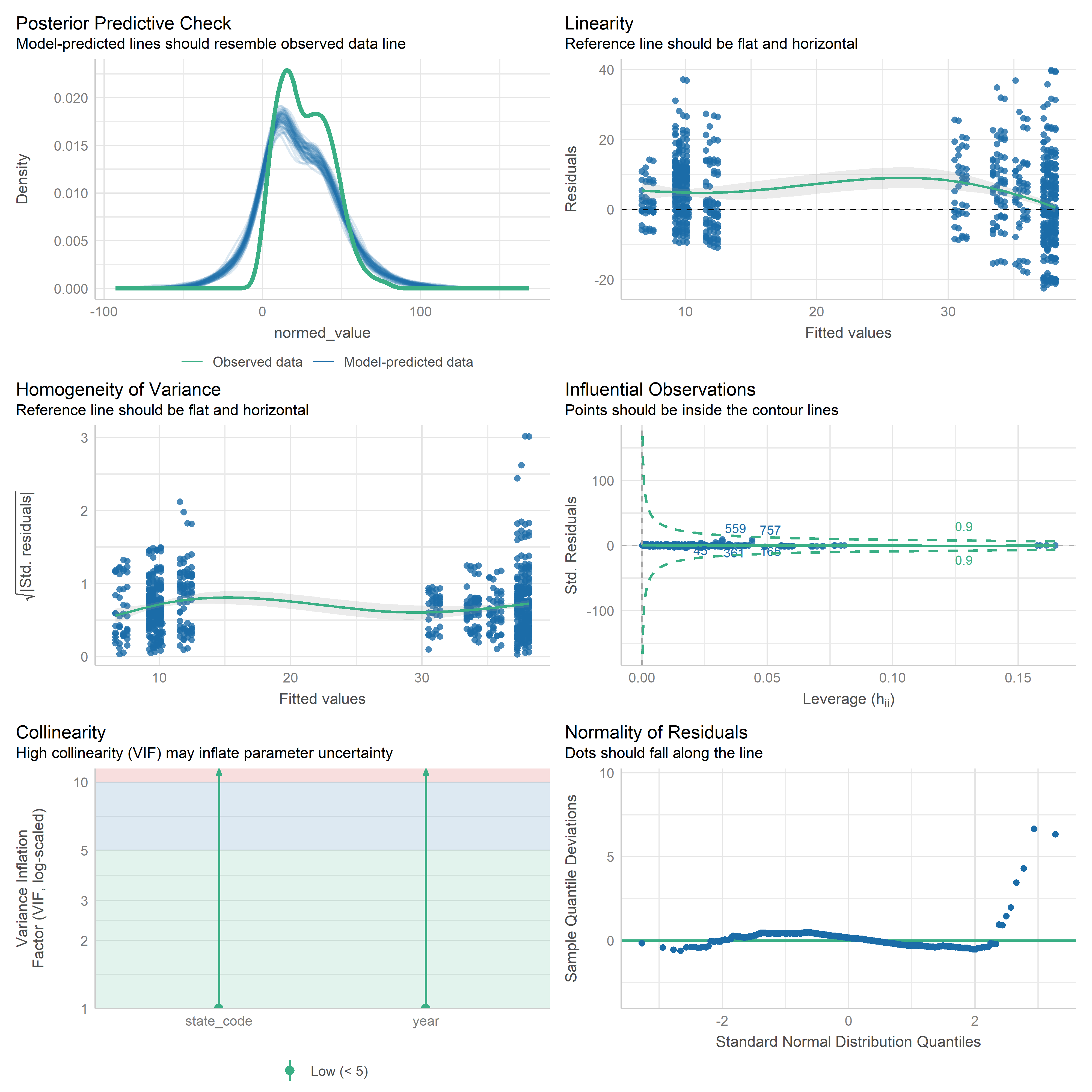
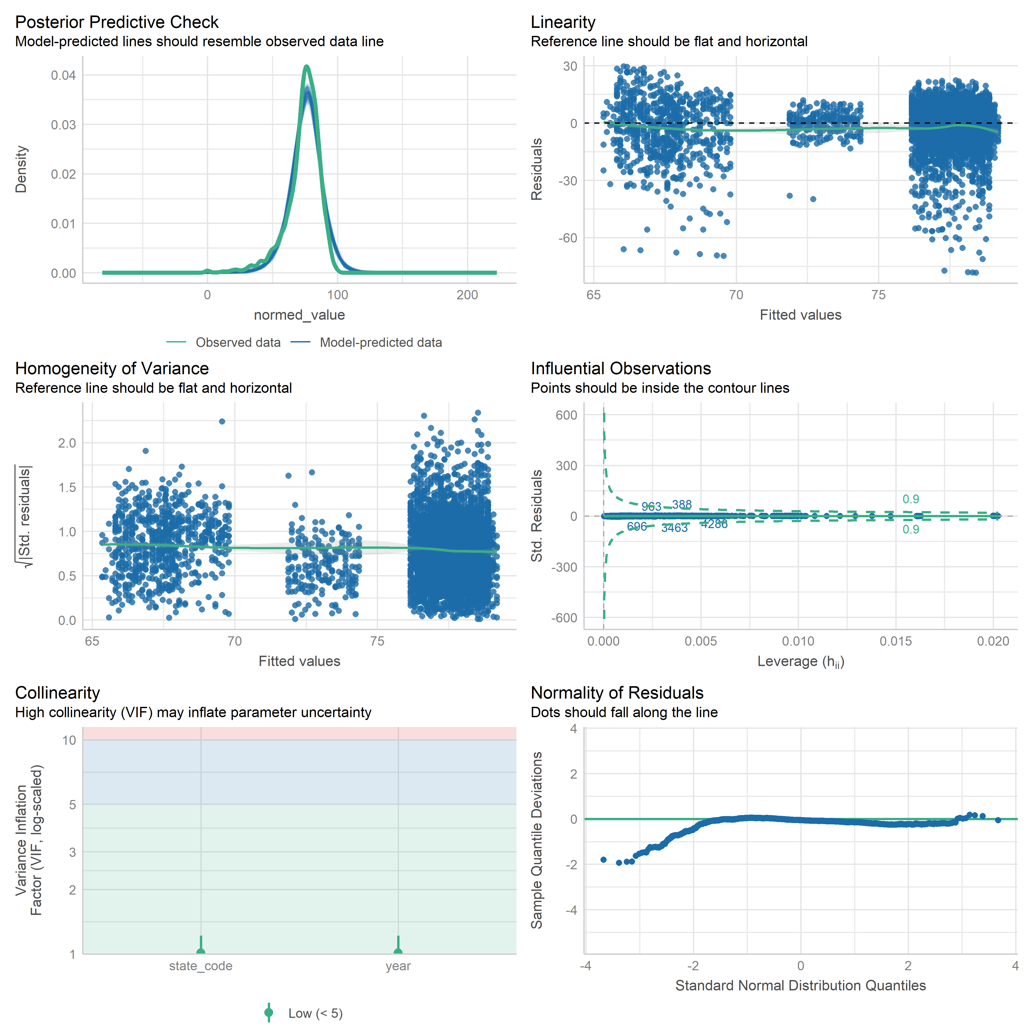
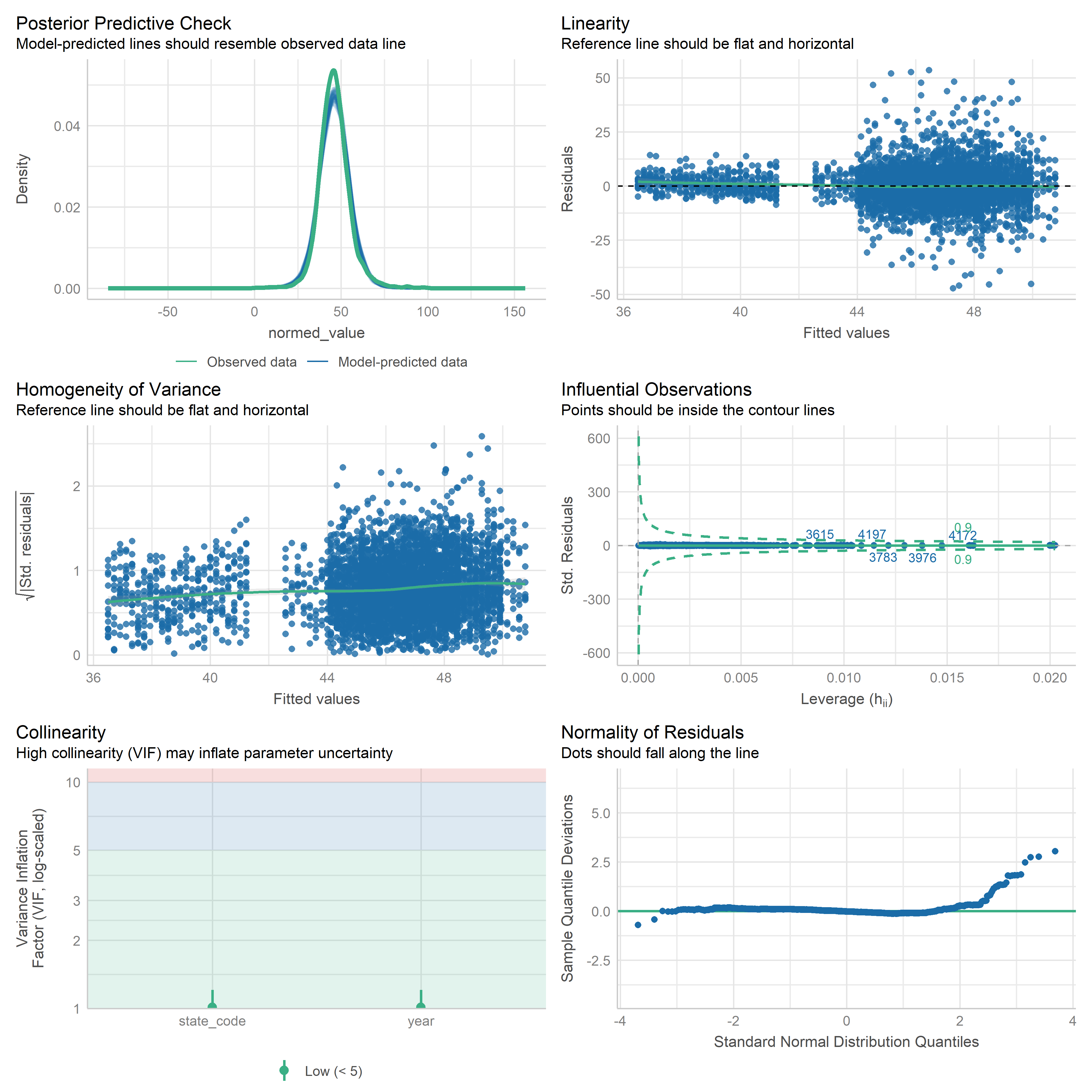
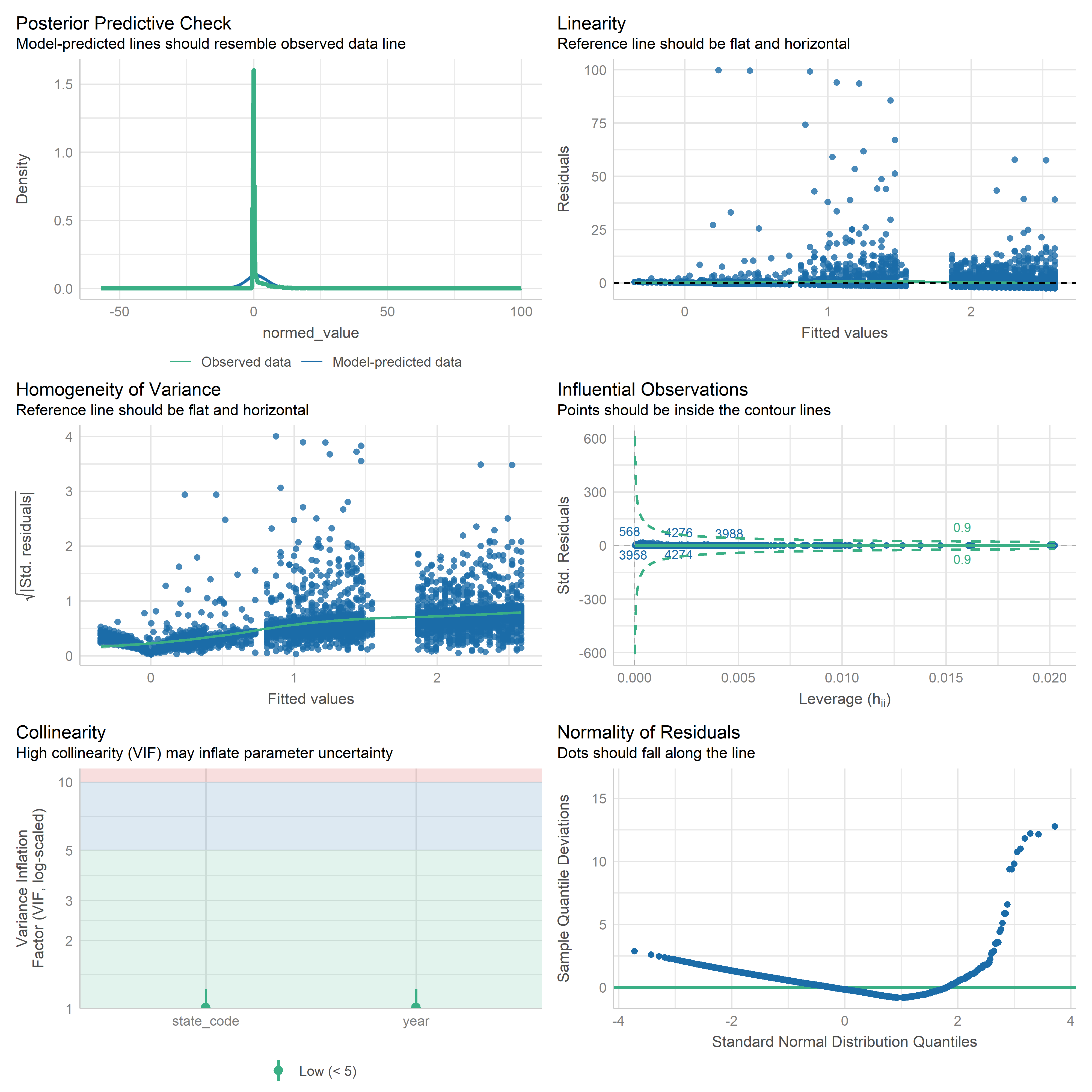
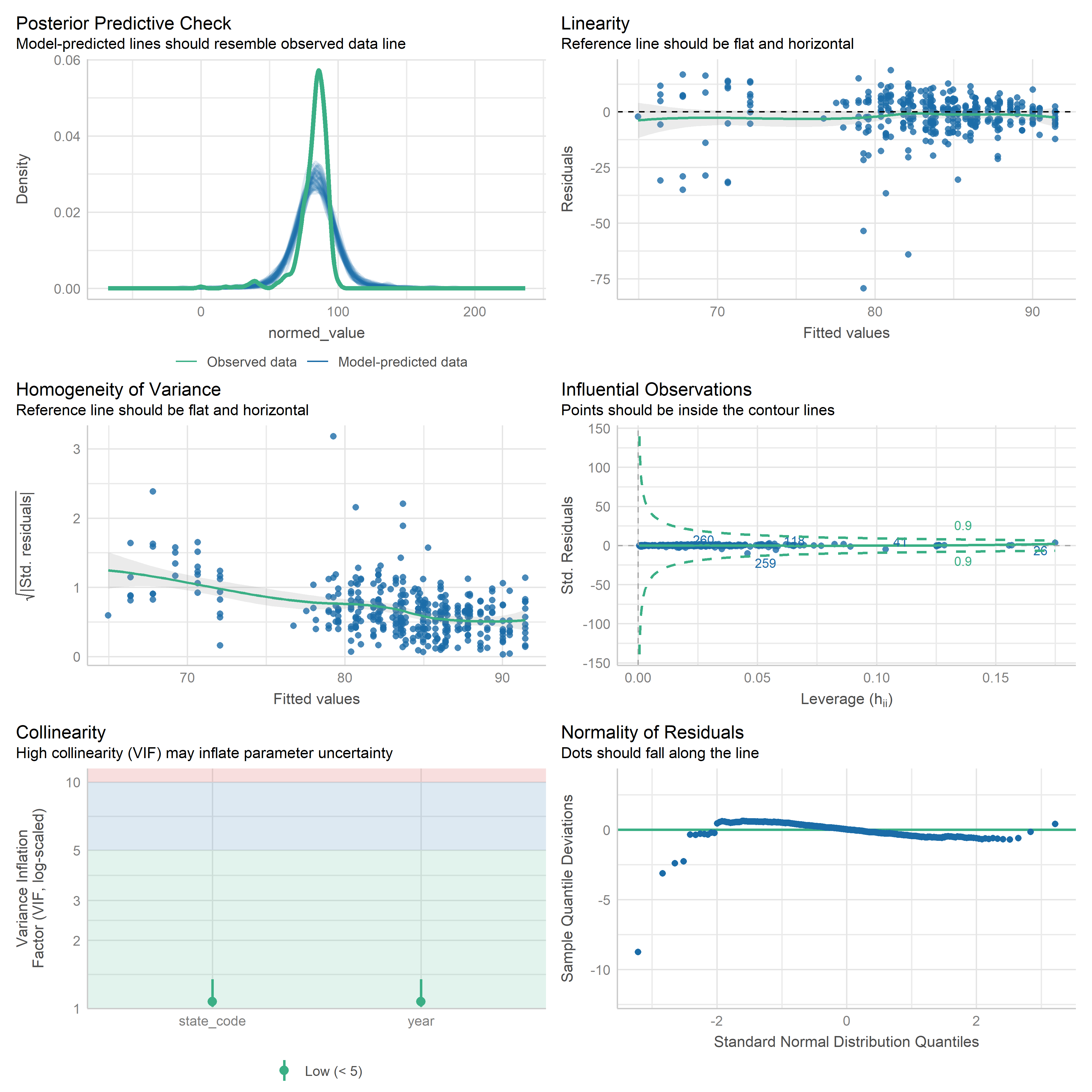
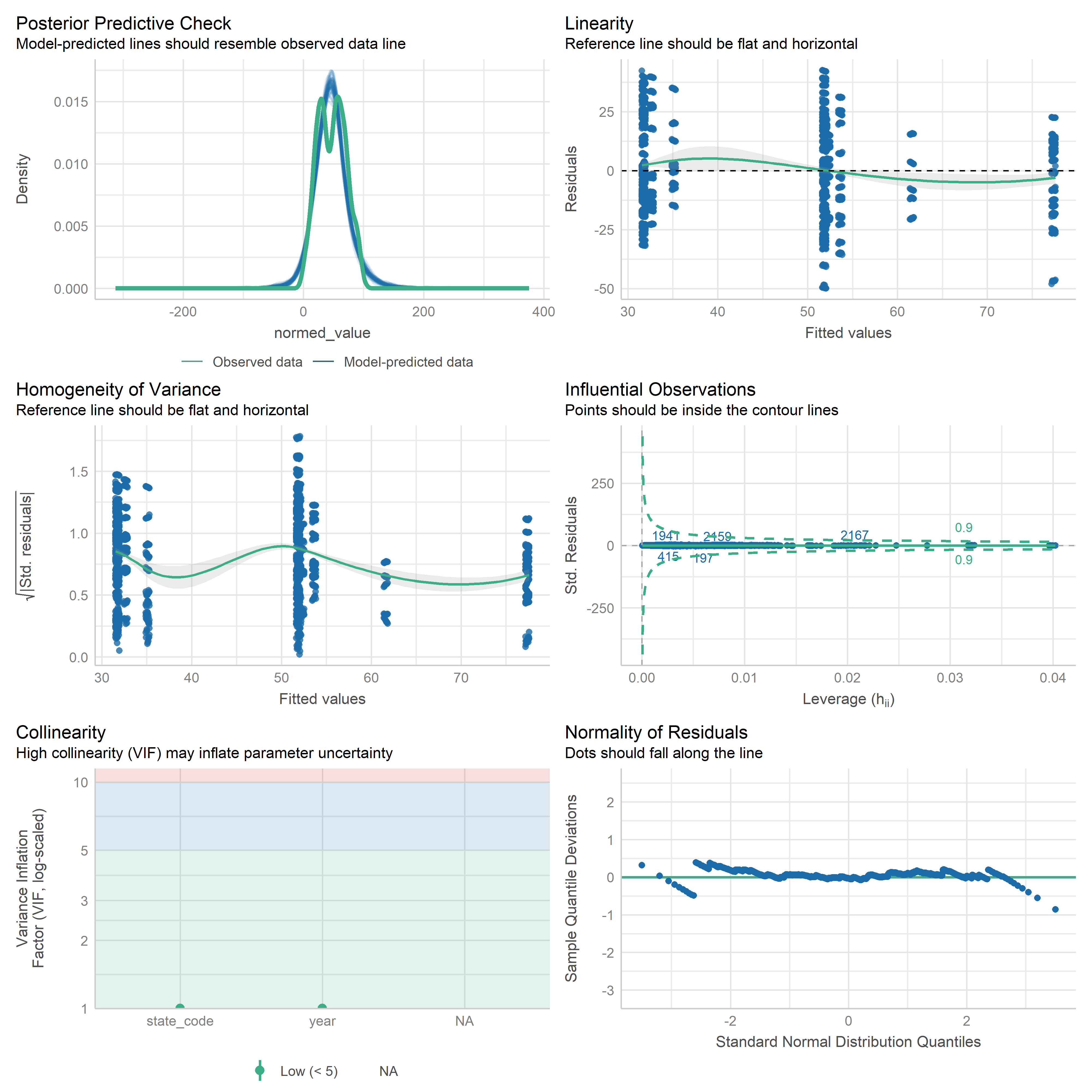
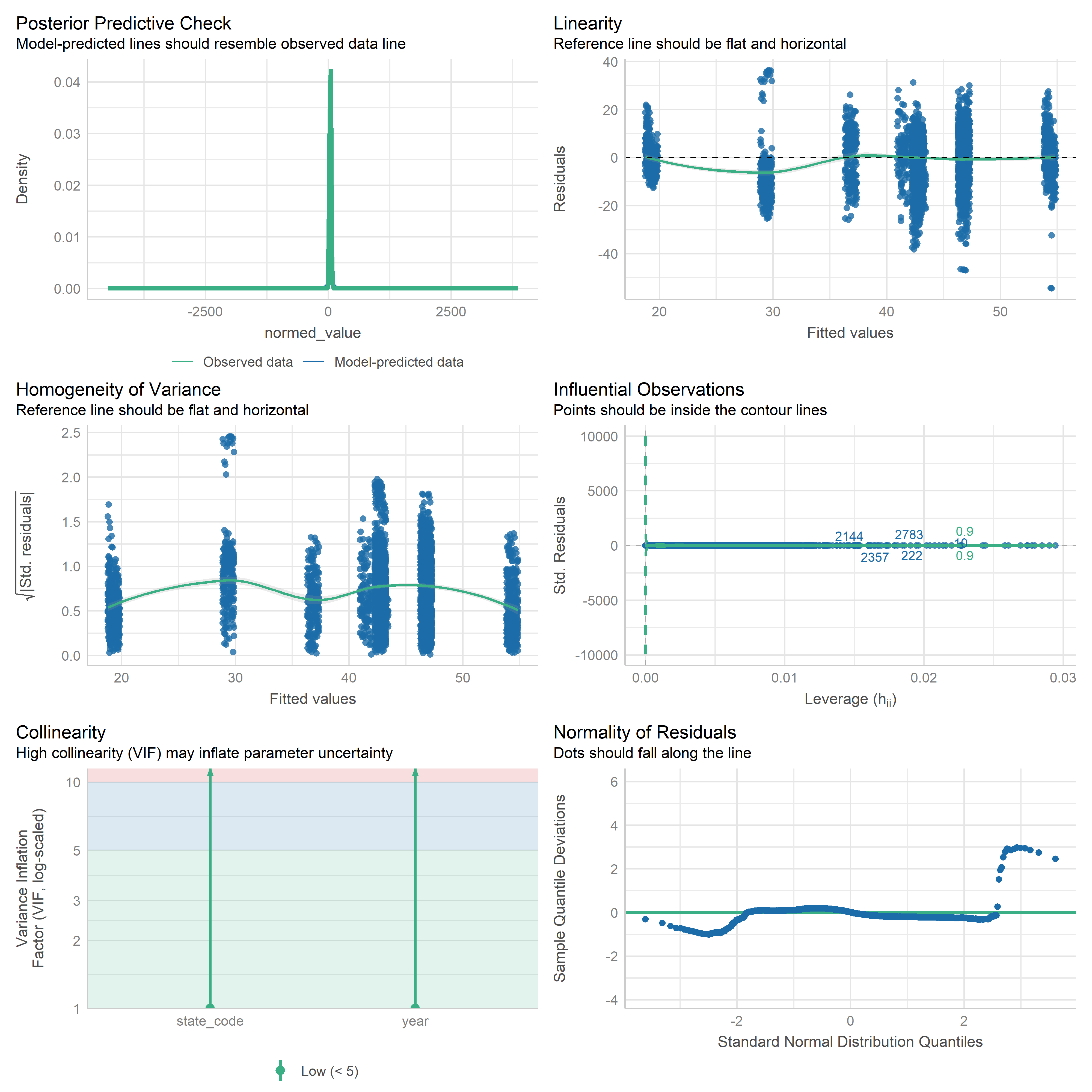
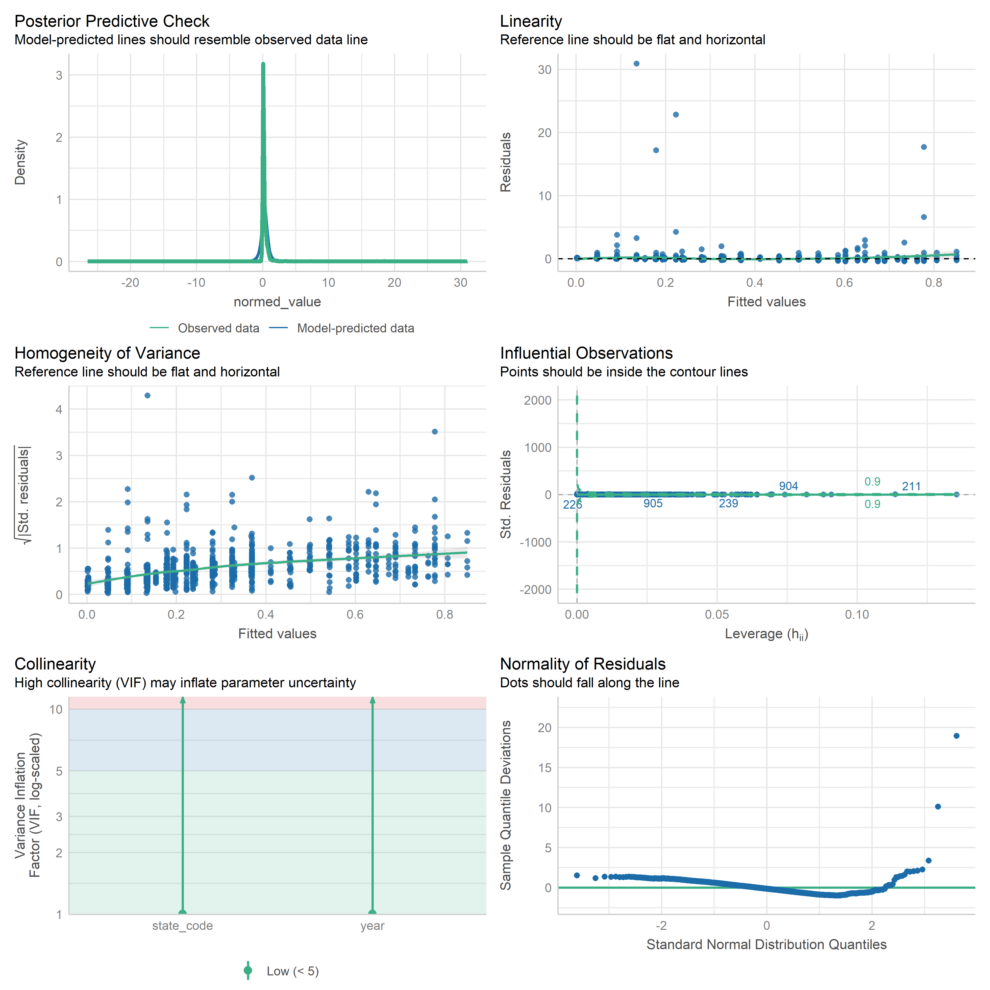
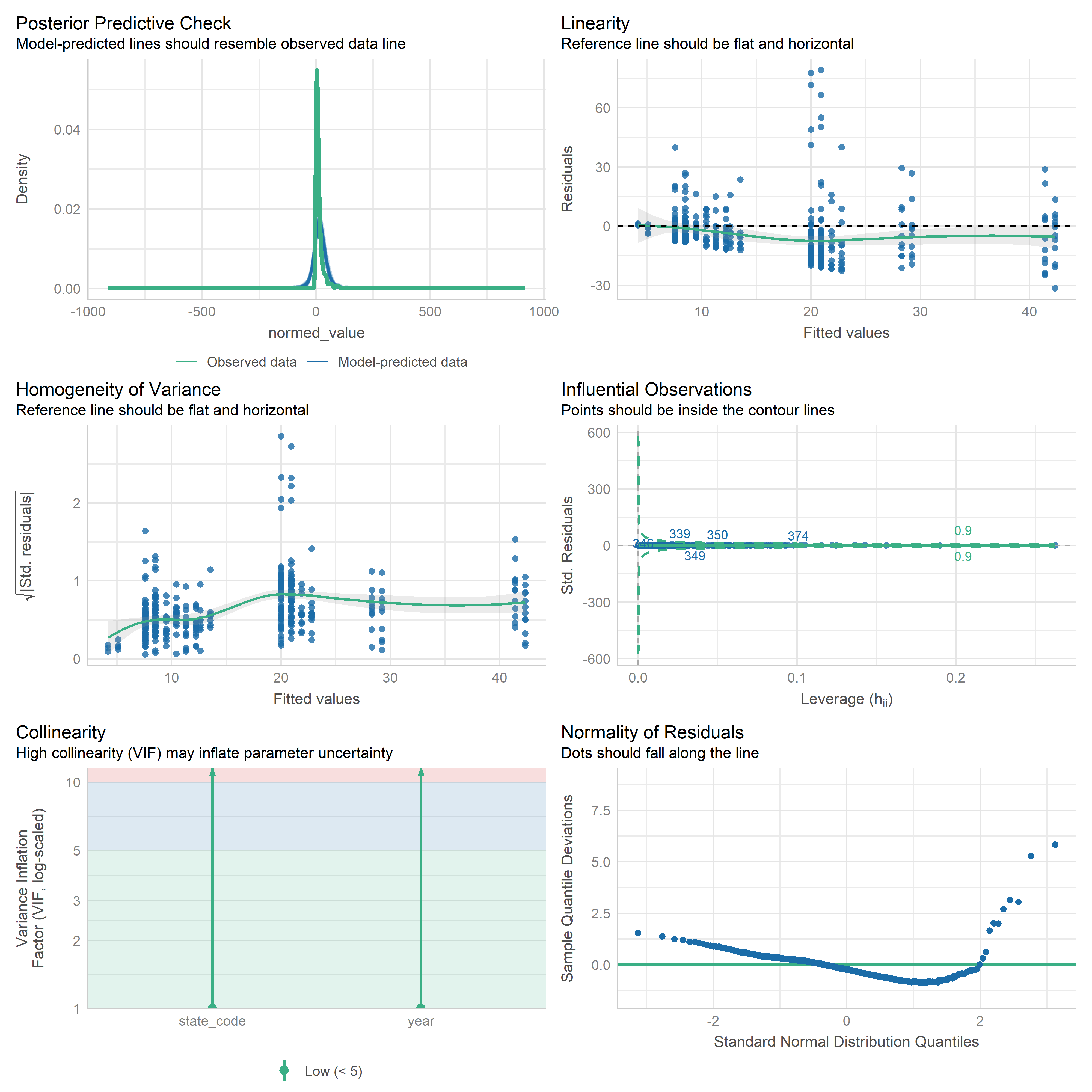
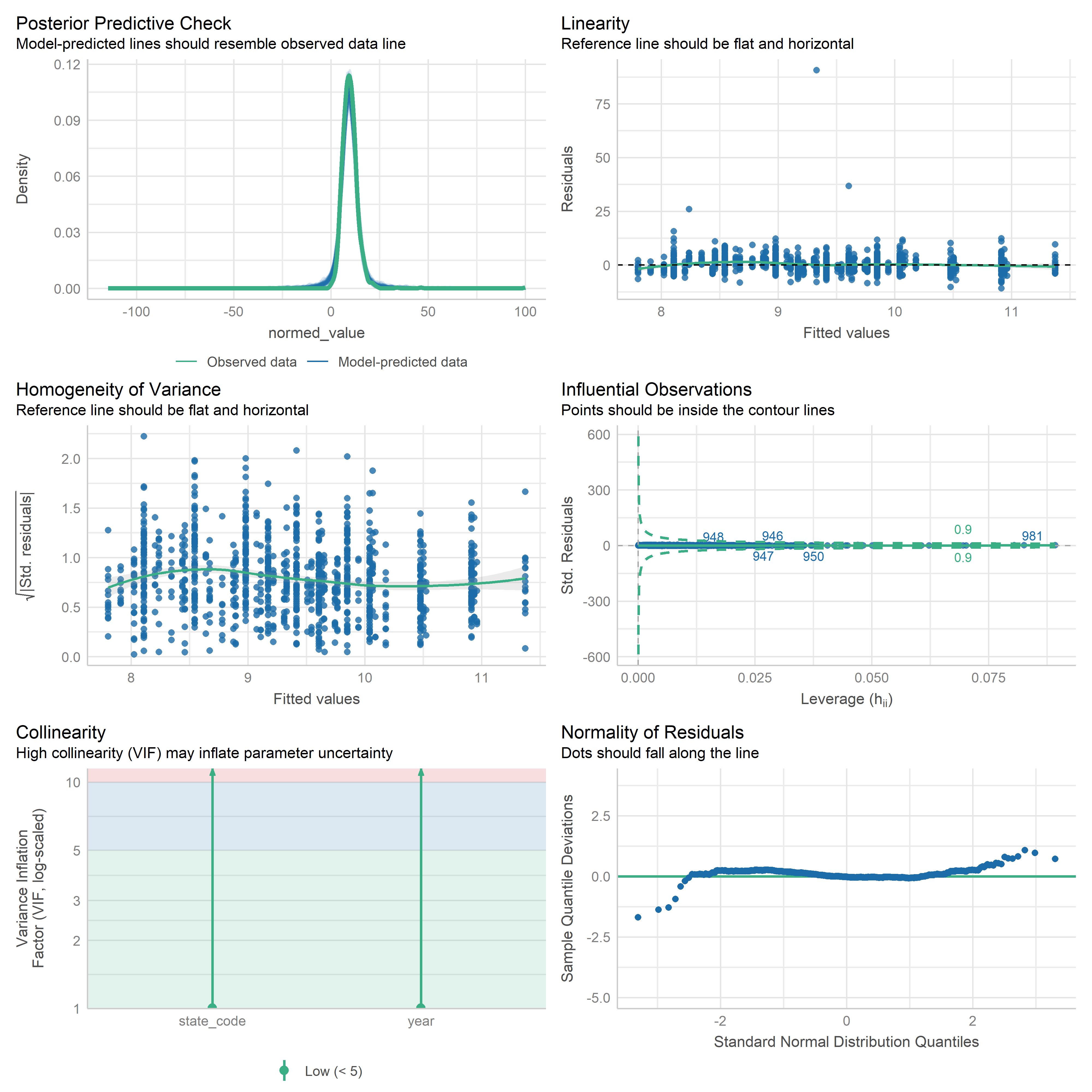
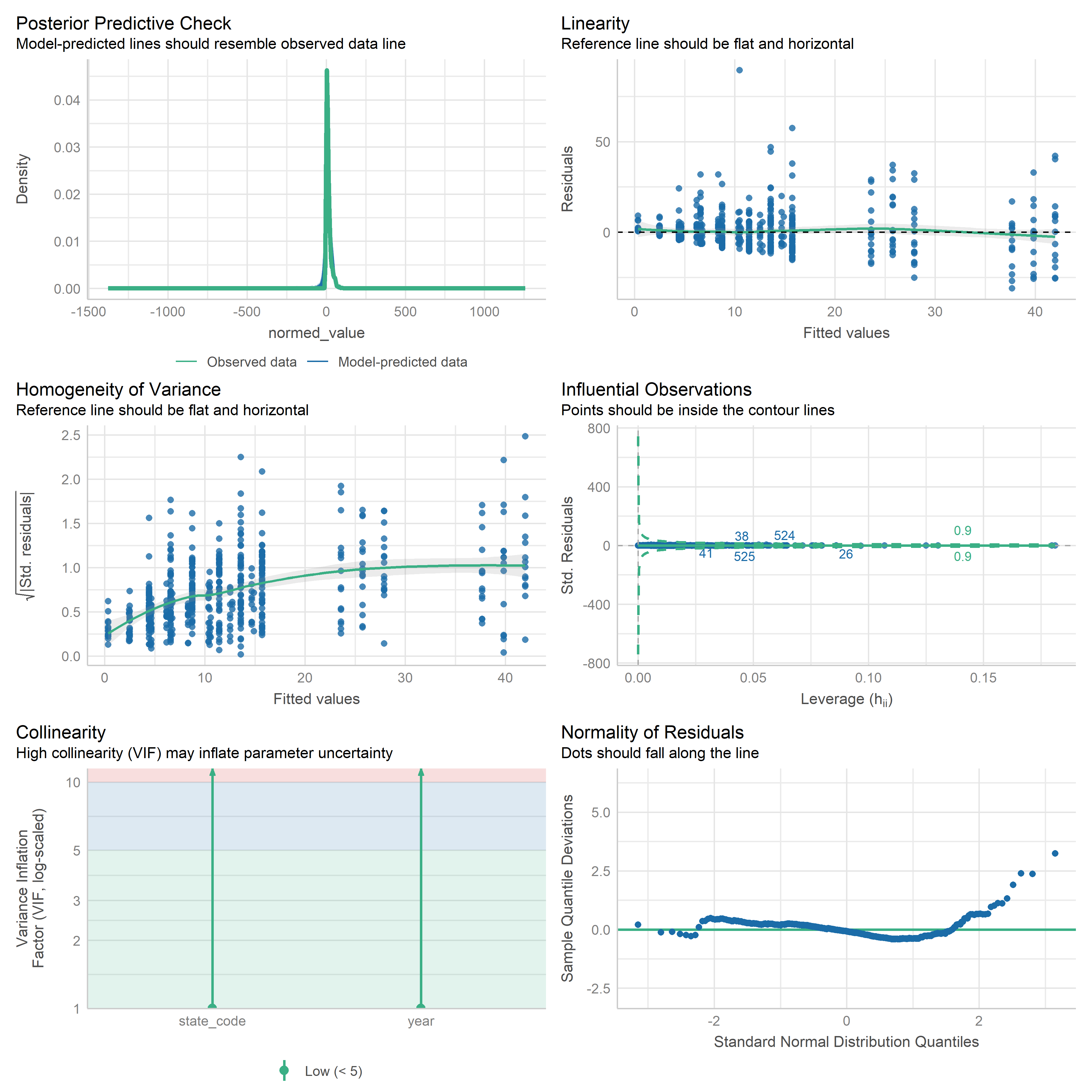
Check residuals of outputs:
Code
res <-readRDS('data/objects/weighted_ols_outs.rds')res_plots <-map(res, ~ {try(performance::check_model(.x))}) %>% purrr::keep(~length(.x) >1)# get_str(res_plots)saveRDS(res_plots, 'data/objects/weighted_ols_residuals.rds')
Now that we have regression outputs, let’s put them in a table to see which ones change significantly over time.
Code
# Put together one table of results from all models, add starsres <-readRDS('data/objects/weighted_ols_outs.rds')get_str(res)# Check for NA outputsres[[1]]$coefficients[['year']]coefs <-map(res, ~ .x$coefficients[['year']])names(coefs[is.na(coefs)])# Mobility disability is NA because there is only 1 year after we join with # weighting variable. So we need to just throw it out if we can't get smoothed# population for 2024.res <- res %>%discard(~is.na(.x$coefficients[[2]]))# testvcov =vcovHC(res[[1]], type ='HC0')test <-coeftest(res[[1]], vcov = vcov)test['year', ]cis <-coefci(res[[1]], vcov. = vcov, level =0.95)cis['year', ]res_df <-imap(res, ~ { vcov =vcovHC(.x, type ='HC0') df <-coeftest(.x, vcov = vcov) %>%tidy() %>%filter(term =='year') %>%mutate(term = .y) conf_ints <-coefci(.x)['year', ] df$ci_low <- conf_ints[1] df$ci_high <- conf_ints[2] df}) %>%bind_rows() %>%mutate(sig =ifelse(p.value <0.05, '*', ''))res_df# How many time series metrics total(n_metrics <-nrow(res_df))# How many change over time significantly( n_change <- res_df %>%filter(sig =='*') %>%nrow())# Percentage significant(perc_sig <-mean(res_df$sig =='*', na.rm =TRUE) *100)
Note that we only have 2 years for the mobility disability metric - 2023 and 2024. But we don’t have a smoothed 5-year population for 2024, only 2023. So we can only use a single year, which means there is no variation in year. So we are dropping this from the analysis.
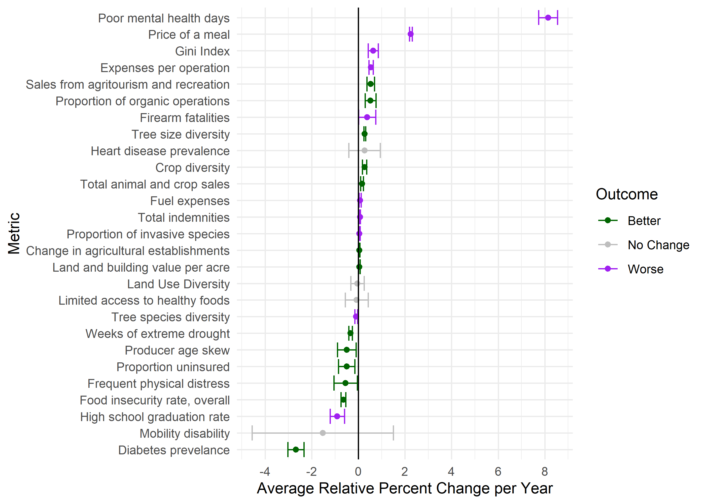
Out of 34 metrics with > 1 time point, we have 23 metrics that change significantly over time (67.65%).
Still have to make sense of the directional values of our metrics. These were defined in the Aggregation from the main analysis branch.
Code
# Of those that are significant, what are trends# leaving in all of them, even if not significant thoughraw_outputs <- res_df %>%mutate(trend =case_when( estimate >0& sig =='*'~'increasing', sig ==''~NA_character_,.default ='decreasing' ))# Bring in directional values. Keep only the ones without question marks, # clearly higher or lowerget_str(data_paper_meta)directions <- data_paper_meta %>%filter(str_detect(desirable, 'higher|lower'), !is.na(variable_name)) %>%mutate(desirable =str_remove_all(desirable, '\\?')) %>%select(variable_name, desirable)reverse <- directions %>%filter(desirable =='lower') %>%pull(variable_name)# Reduce to only vars that have a direction.# Here we lose a few metricsmodel_outputs <- raw_outputs %>%filter(term %in% directions$variable_name) %>%mutate(reverse =ifelse(term %in% reverse, TRUE, FALSE),outcome =case_when( reverse ==FALSE& trend =='increasing'~'better', reverse ==FALSE& trend =='decreasing'~'worse', reverse ==TRUE& trend =='increasing'~'worse', reverse ==TRUE& trend =='decreasing'~'better',.default =NA ),across(where(is.numeric), ~format(round(.x, 3), nsmall =3)) )model_outputs# See what we lost(lost <-setdiff(raw_outputs$term, model_outputs$term))(n_lost <-length(lost))(print_lost <- lost %>%paste0(collapse =', '))# proportion getting better or worse(tab <-table(model_outputs$outcome))(percs <-round(prop.table(tab), 3) *100)
62.1% are getting better and 37.9% are getting worse. We drop 3 metrics here that don’t have proper directions (vacancyRate, annualPrecipMM, ftmProdRatio).
Check out table with outputs for each regression. Filter by significance and outcome. Trend is just whether it is going up or down, outcome is whether that is good or bad.
1.3 Table
Code
## Add framework infoframed_outputs <- data_paper_meta %>%select(dimension, index, indicator, metric, variable_name) %>%right_join(model_outputs, by =join_by(variable_name == term))## Save some outputs for paper# Raw csv for referencewrite_csv( framed_outputs,'outputs/lm_reg_outputs.csv')# Make table for Wordframed_outputs %>%select(-c( dimension, index, indicator, variable_name, trend, reverse, sig,starts_with('ci') )) %>%flextable() %>% flextable::font(part ="all", fontname ="Times New Roman") %>%save_as_docx(path ='outputs/lm_reg_outputs.docx' )## Create interactive table for Quartoget_reactable( framed_outputs, defaultPageSize =10,columns =list(variable_name =colDef(minWidth =200),sig =colDef(minWidth =50),reverse =colDef(minWidth =75),statistic =colDef(minWidth =75),outcome =colDef(minWidth =75) ))
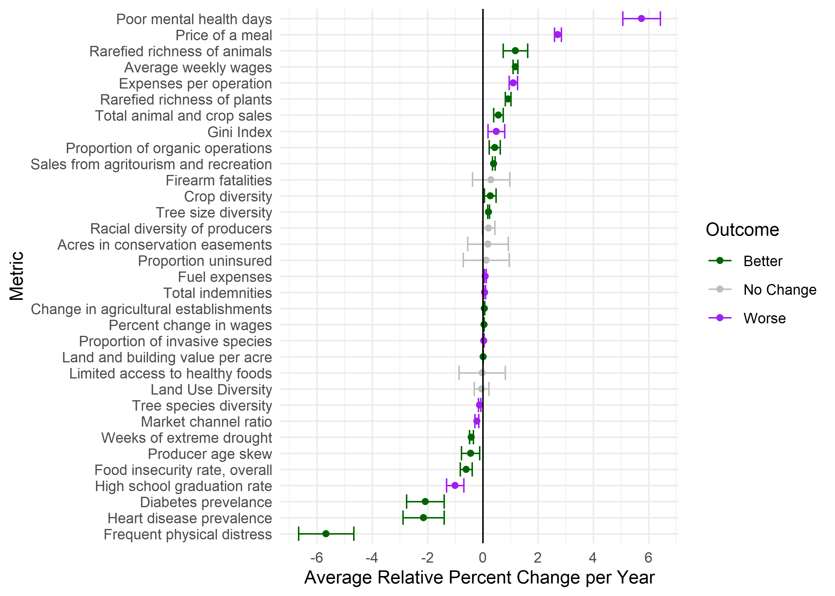
1.4 Figure
Figure below shows 95% confidence intervals for the coefficients of each metric, including state as a covariate.
spatialreg for spatially weighted regressions, but not panels. First trying a single example with gini. Note that because Census data spans the change in administrative boundaries in CT, we can’t use CT at all here.
Code
get_str(datasets$dp_metrics_county)dat <- datasets$dp_metrics_county %>%pivot_wider(id_cols = fips:year,names_from = variable_name,values_from = value )get_str(dat)# Remove CT. Drop na ginis, but, get complete cases for relevant fips and yearsdat <- dat %>%select(fips, year, gini) %>%mutate(gini_normed =min_max(gini)) %>%filter(str_detect(fips, '^09', negate =TRUE)) %>%drop_na(gini) %>%complete(fips, year)get_str(dat)# List weightslw <- neast_counties_2024 %>%right_join(dat) %>%select(fips, year, gini) %>%poly2nb() %>%nb2listw(zero.policy =TRUE)# Regular weightsget_str(weights_crosswalk)weight_var <- weights_crosswalk$weight_variable[weights_crosswalk$variable_name =='gini']weight_df <- datasets$dp_weights# if (!is.na(weight_var) && length(weight_var) > 0) {# weight_df <- weight_df %>% # filter(variable_name == weight_var)# }weight_df <- weight_df %>%mutate(value =as.numeric(value), year =as.numeric(year) ) %>%rename(weight_value = value, weight_name = variable_name,weight_year = year ) %>%filter(weight_name == weight_var, str_length(fips) ==5)get_str(weight_df)get_str(dat)dat <-left_join(dat, weight_df, by =join_by(fips, year == weight_year)) %>%distinct()get_str(dat)# Run regressionsar <-errorsarlm( gini_normed ~ year,data = dat,listw = lw,weight = weight_value)
Code
summary(sar)
Call:errorsarlm(formula = gini_normed ~ year, data = dat, listw = lw,
    weights = weight_value)

Residuals:
     Min       1Q   Median       3Q      Max
-36.0447 -17.4249 -11.0732  -3.2657  54.2701

Type: error
Coefficients: (asymptotic standard errors)
              Estimate Std. Error z value Pr(>|z|)
(Intercept) -938.81700  309.60177 -3.0323 0.002427
year           0.49176    0.15341  3.2055 0.001348

Lambda: 0.50321, LR test value: 31.78, p-value: 0.000000017264
Approximate (numerical Hessian) standard error: 0.080826
    z-value: 6.2258, p-value: 0.00000000047902
Wald statistic: 38.761, p-value: 0.00000000047902

Log likelihood: -2891.242 for error model
ML residual variance (sigma squared): 66033000, (sigma: 8126.1)
Number of observations: 627
Number of parameters estimated: 4
AIC: 5790.5, (AIC for lm: 5820.3)
2.2 All Models
Use errorsarlm on all metrics.
Code
get_str(datasets$dp_metrics_county)state_link <- fips_key %>%filter(str_length(fips) ==2, fips !='00') %>%select(fips, state_code)dat <- datasets$dp_metrics_county %>%pivot_wider(id_cols = fips:year,names_from = variable_name,values_from = value ) %>%filter(str_detect(fips, '^09', negate =TRUE)) %>%mutate(link =str_sub(fips, end =2)) %>%left_join(state_link, by =join_by(link == fips)) %>%select(-link)get_str(dat)# Get vector of vars(vars <-names(dat)[!names(dat) %in%c('fips', 'year', 'state_code')])tic()get_time()plan(multisession, workers =availableCores(omit =2))out <-future_map(vars, \(var) {# out <- map(vars[1], \(var) {cat('\n\nStarting', var)tryCatch({# Reduce to relevant variable, remove NAs df <- dat %>%select(fips, year, !!sym(var), state_code) %>%drop_na(!!sym(var)) %>%mutate(normed =min_max(!!sym(var)))# Regular weights weight_var <- weights_crosswalk$weight_variable[weights_crosswalk$variable_name == var] weight_df <- datasets$dp_weights# if (!is.na(weight_var) && length(weight_var) > 0) {# weight_df <- weight_df %>% # filter(variable_name == weight_var)# } weight_df <- weight_df %>%mutate(value =as.numeric(value), year =as.numeric(year) ) %>%rename(weight_value = value, weight_name = variable_name,weight_year = year ) %>%filter(weight_name == weight_var, str_length(fips) ==5) df <- df %>%inner_join(weight_df, by =join_by(fips, year == weight_year))# distinct()cat('\nJoined to weights')# List weights lw <- neast_counties_2024 %>%right_join(df) %>%select(fips, year, normed) %>%poly2nb() %>%nb2listw(zero.policy =TRUE) cat('\nCreated lw')# Run error sar model# formula <- as.formula(paste(var, "~ as.numeric(year) + state_code")) model <-errorsarlm( normed ~as.numeric(year) + state_code,data = df,listw = lw,weights = weight_value ) cat('\nRan model')return(model) },error =function(e) {return(paste0('Error with ', var, ': ', e)) } )}, .progress =FALSE) %>%setNames(c(vars))plan(sequential)toc()# 6 to 12 minutes or sooutout[[1]]get_str(out)map(out, class)# get_str(out[[1]])# map(out, ~ .x['fips'])# map(out, ~ summary(.x))saveRDS(out, 'data/objects/errorsarlm_weighted_outs.rds')
2.2.1 Table
Code
sar_outs <-readRDS('data/objects/errorsarlm_outs.rds')# sar_outs <- readRDS('data/objects/errorsarlm_weighted_outs.rds')sar_outs <- sar_outs[names(sar_outs) !='state_code'] %>%keep(~class(.x) =='Sarlm')get_str(sar_outs, 1)get_str(sar_outs[[1]])summary(sar_outs[[1]])sum <-summary(sar_outs[[1]])tidy(sum)# # No robust errors hereconfint(sar_outs[[1]])# confint(sar_outs[[1]])[3, ]# confints <- confint(sar_outs[[2]])[3, ]sar_df <-imap(sar_outs, ~ {tryCatch( { confints <-confint(.x)[3, ] out <- .x %>%tidy() %>%filter(str_detect(term, 'year')) %>%mutate(variable_name = .y,conf_low = confints[1],conf_high = confints[2] ) %>%select(-term) %>%mutate(sig =ifelse(p.value <0.05, '*', ' ') %>%as.character()) return(out) },error =function(e) {message('Error')print(e) } )})sar_df <- sar_df %>%keep(is.data.frame) %>%bind_rows()# get_str(sar_df)# sar_dfsar_raw_outputs <- sar_df %>%mutate(trend =case_when( estimate >0& sig =='*'~'increasing', sig ==''~NA_character_,.default ='decreasing' ))# get_str(sar_raw_outputs)# sar_raw_outputs# Bring in directional values. Keep only the ones without question marks, # clearly higher or lowerget_str(data_paper_meta)directions <- data_paper_meta %>%filter(str_detect(desirable, 'higher|lower'), !is.na(variable_name)) %>%mutate(desirable =str_remove_all(desirable, '\\?')) %>%select(variable_name, desirable)reverse <- directions %>%filter(desirable =='lower') %>%pull(variable_name)# Reduce to only vars that have a direction.# Here we lose a few metricssar_model_outputs <- sar_raw_outputs %>%filter(variable_name %in% directions$variable_name) %>%mutate(reverse =ifelse(variable_name %in% reverse, TRUE, FALSE),outcome =case_when( reverse ==FALSE& trend =='increasing'~'better', reverse ==FALSE& trend =='decreasing'~'worse', reverse ==TRUE& trend =='increasing'~'worse', reverse ==TRUE& trend =='decreasing'~'better',.default =NA ),outcome =ifelse(sig !='*', NA, outcome),across(where(is.numeric), ~format(round(.x, 3), nsmall =3)) )sar_model_outputs(n_metrics <-dim(sar_model_outputs)[1])# See what we lost(lost <-setdiff(sar_raw_outputs$variable_name, sar_model_outputs$variable_name))(n_lost <-length(lost))(print_lost <- lost %>%paste0(collapse =', '))# proportion getting better or worse(tab <-get_table(sar_model_outputs$outcome))(percs <-round(prop.table(tab), 3) *100)
We have 30 metrics modeled. 50% are getting better, 33.3% are getting worse, and 16.7% are stable. We drop 3 metrics here that don’t have proper directions (vacancyRate, populationChangePerc, annualPrecipMM).
Code
sar_framed_outputs <- data_paper_meta %>%select(dimension, index, indicator, metric, variable_name) %>%right_join(sar_model_outputs, by =join_by(variable_name == variable_name))## Save some outputs for paper# Raw csv for referencewrite_csv( sar_framed_outputs,'outputs/errorsar_reg_outputs.csv')# Make table for Word# framed_outputs %>% # select(-c(# dimension,# index, # indicator,# variable_name,# trend,# reverse,# sig,# starts_with('ci')# )) %>% # flextable() %>% # flextable::font(part = "all", fontname = "Times New Roman") %>% # save_as_docx(# path = 'outputs/lm_reg_outputs.docx'# )## Create interactive table for Quartoget_reactable( sar_framed_outputs, defaultPageSize =10,columns =list(variable_name =colDef(minWidth =200),sig =colDef(minWidth =50),reverse =colDef(minWidth =75),statistic =colDef(minWidth =75),outcome =colDef(minWidth =75) ))
Trying splm package for spatially weighted panel models. This is not going well though - too much missing data means it is very difficult to get a balanced panel.
Code
get_str(datasets$dp_metrics_county)dat <- datasets$dp_metrics_county %>%pivot_wider(id_cols = fips:year,names_from = variable_name,values_from = value )get_str(dat)# Get rid of geometry, make our df a plm objectdf <- dat %>%select(fips, year, gini) %>%# select(fips, year, otyAnnualAvgEstabsCountPctChgNAICS11) %>%filter(str_detect(fips, '^09', negate =TRUE)) %>%na.omit() %>% plm::pdata.frame()get_str(df)df %>%group_by(year, fips) %>%summarize(n()) %>%arrange(year, fips) %>%print(n =500)# Get balanced fipsall_years <-sort(unique(df$year))balanced_fips <- df %>%group_by(fips) %>%filter(setequal(sort(year), all_years)) %>%pull(fips) %>%unique()df <- df %>%filter(fips %in% balanced_fips)# Get our listw based on countieslw <- neast_counties_2024 %>%filter(fips %in% df$fips) %>%poly2nb() %>%nb2listw(zero.policy =TRUE)# Pooling modelpool <-spml( gini ~as.numeric(year),data = df, listw = lw,model ='pooling')summary(pool)# Try FE error modelfe_err <-spml( gini ~as.numeric(year),data = df, listw = lw,model ='within')summary(fe_err)# RE error modelre_err <-spml( gini ~as.numeric(year), data = df, listw = lw,model ='random')summary(re_err)# Try lagsarlmlagsar <-lagsarlm(# otyAnnualAvgEstabsCountPctChgNAICS11 ~ as.numeric(year), gini ~as.numeric(year),data = df,listw = lw)summary(lagsar)# # Check to use RE or FE, see whether x_it related to a_i (idiosyncratic error)# test <- sphtest(fe_err, re_err)# test# # Not sig: use RE, more efficient# # # Check RE output# summary(re_err)
3.2 All Models
Code
get_str(datasets$dp_county_wide)dat <- datasets$dp_county_wide %>%select(fips, year, any_of(datasets$series_vars))get_str(dat)# Get vector of varsvars <-names(dat)[!names(dat) %in%c('fips', 'year')]# Map over each var and do steps 1 through 5out <-map(vars, \(var) {cat('\n\nStarting', var)tryCatch({# Reduce to relevant variable, remove NAs df <- dat %>%select(fips, year, !!sym(var)) %>%filter(str_detect(fips, '^09', negate =TRUE)) %>%na.omit()# complete(fips, year)# mutate(!!sym(var) := ifelse(is.na(!!sym(var)), 0, !!sym(var)))# 1. Only use fips that produce balanced panel balanced_fips <- df %>%group_by(fips) %>%filter(n() ==length(unique(df$year))) %>%pull(fips) %>%unique() df <- df %>%filter(fips %in% balanced_fips)# 2. Create lw object lw <- neast_counties_2024 %>%filter(fips %in% balanced_fips) %>%# filter(fips %in% df$fips) %>%poly2nb() %>%nb2listw(zero.policy =TRUE)cat('\nCreated lw')# Make df a plm object df <- plm::pdata.frame(df)# 3. Run pooled panel model formula <-as.formula(paste(var, "~ as.numeric(year)")) model <-spml( formula,data = df,listw = lw,index =c('fips', 'year'),model ='pooling',spatial.error ='b'# lag = TRUE )cat('\nRan model')return(list('model'= model, 'fips'= balanced_fips)) },error =function(e) {return(paste0('Error with ', var, ': ', e)) } )}, .progress =FALSE) %>%setNames(c(vars))outget_str(out)get_str(out[[1]])summary(out[[1]]$model)map(out, ~ .x['fips'])map(out, ~summary(.x[[1]]))# Save for posteritysaveRDS(out, 'data/objects/spatial_regression_outs.rds')
3.3 All Models Weighted
Code
# TODO: fix this. we broke it here somewhere.get_str(datasets$dp_county_wide)dat <- datasets$dp_county_wide %>%select(fips, year, any_of(datasets$series_vars))get_str(dat)# Get vector of varsvars <-names(dat)[!names(dat) %in%c('fips', 'year')]## Normalizationget_str(dat)dat <- dat %>%mutate(across(all_of(vars), ~min_max(.x)))get_str(dat) map(dat, ~range(.x, na.rm =TRUE))## Regressionsout <-map(vars, \(var) {# out <- map('treeDiversity', \(var) {cat('\n\nStarting', var)tryCatch({# Reduce to relevant variable, remove NAs df <- dat %>%select(fips, year, !!sym(var)) %>%filter(str_detect(fips, '^09', negate =TRUE)) %>%na.omit()## Add weights weight_var <- weights_crosswalk$weight_variable[weights_crosswalk$variable_name == var] weight_df <- datasets$dp_weightsif (!is.na(weight_var) &&length(weight_var) >0) { weight_df <- weight_df %>%filter(variable_name == weight_var) } weight_df <- weight_df %>%mutate(value =as.numeric(value),year =as.numeric(year) ) %>%rename(weight_value = value,weight_name = variable_name,weight_year = year )# Do join depending on whether weight var has a yearif (all(is.na(weight_df$weight_year))) { df <- df %>%inner_join(weight_df, by =join_by(fips)) } else { df <- df %>%inner_join(weight_df, by =join_by(fips, year == weight_year)) }# Weight the variable appropriately var_weighted <-paste0(var, '_weighted') df <- df %>%mutate(!!sym(var_weighted) :=!!sym(var) *sqrt(weight_value)) %>%drop_na(!!sym(var_weighted))## Only use fips that produce balanced panel balanced_fips <- df %>%group_by(fips) %>%filter(n() ==length(unique(df$year))) %>%pull(fips) %>%unique() df <- df %>%filter(fips %in% balanced_fips)## Create lw object lw <- neast_counties_2024 %>%filter(fips %in% balanced_fips) %>%filter(fips %in% df$fips) %>%poly2nb() %>%nb2listw(zero.policy =TRUE)cat('\nCreated lw')## Run pooled panel model df <- plm::pdata.frame(df)# formula <- as.formula(paste(var_weighted, "~ as.numeric(year)")) formula <-as.formula(paste(var_weighted, "~ as.numeric(year)")) model <-spml( formula,data = df,listw = lw,index =c('fips', 'year'),model ='pooling' )cat('\nRan model')return(list('model'= model, 'fips'= balanced_fips)) },error =function(e) {return(paste0('Error with ', var, ': ', e)) } )}, .progress =FALSE) %>%setNames(c(vars))outout[[2]]out$cropDiversity # check for smoothed weighting varget_str(out)get_str(out[[1]])summary(out$gini$model)map(out, ~ .x['fips'])map(out, ~summary(.x[[1]]))# Getting errors because there are NO balanced fips# Save for posteritysaveRDS(out, 'data/objects/spatial_panel_outs.rds')
Check how they turned out:
Code
out <-readRDS('data/objects/spatial_panel_outs.rds')get_str(out)# How many were successful(perc_success <-mean(map(out, class) =='list') *100)# Check out errors onlyerrors <- out %>%keep(is.character)errors(error_vars <-names(errors))
model_outs <- out %>%keep(is.list)# Make a tablespatial_table <-imap(model_outs, ~ {tryCatch({# Pull model output results and coefficients sum <-summary(.x[[1]]) coefs <- sum$CoefTable[2, ]# Add confidence intervals conf_ints <-confint(.x[[1]])[2, ] %>%as.vector()# df$ci_low <- conf_ints[1]# df$ci_high <- conf_ints[2] df <-data.frame(n =length(.x$fips),# type = .x[[1]]$type,var = .y,# phi = sum$errcomp[1],rho = sum$ErrCompTable[[1]],est = coefs[1],se = coefs[2],t = coefs[3],ci_low = conf_ints[1],ci_high = conf_ints[2],p = coefs[4] ) # Figure out good or bad outcome# If sig, then check reverse. else blank# If reverse, reverse it, else same# If up, good, else bad df <- df %>%mutate(sig =ifelse(p <0.05, TRUE, FALSE),posneg =case_when( est >0~'pos', est <0~'neg',.default ='' ),reverse =ifelse(.y %in% reverse, TRUE, FALSE),direction =case_when( sig ==TRUE& reverse ==TRUE& posneg =='pos'~'neg', sig ==TRUE& reverse ==TRUE& posneg =='neg'~'pos', sig ==TRUE& reverse ==FALSE~as.character(posneg),.default ='' ),outcome =case_when( sig ==FALSE~'', sig ==TRUE& direction =='pos'~'better', sig ==TRUE& direction =='neg'~'worse',.default ='-' ) ) %>%select(-c(posneg, direction))return(df) },error =function(e) {return(paste('Error:', e)) } )}) %>%bind_rows()# get_str(spatial_table)## Make table for Wordspatial_table %>%select(n:t, p, outcome) %>%mutate(across(c(rho:p), ~format(round(.x, 3), nsmall =3))) %>%flextable() %>% flextable::font(part ="all", fontname ="Times New Roman") %>%save_as_docx(path ='outputs/spatial_reg_outputs.docx' )## Round off and make table for Quartospatial_table %>%mutate(across(c(rho:p), ~format(round(.x, 3), nsmall =3)) ) %>%get_reactable(defaultColDef =colDef(minWidth =50),columns =list(n =colDef(minWidth =50),var =colDef(minWidth =200),est =colDef(minWidth =100,name ='β' ),outcome =colDef(minWidth =75),rho =colDef(name ='ρ'),p =colDef(name ='p-value'),'p-value'=colDef(minWidth =100) ) )
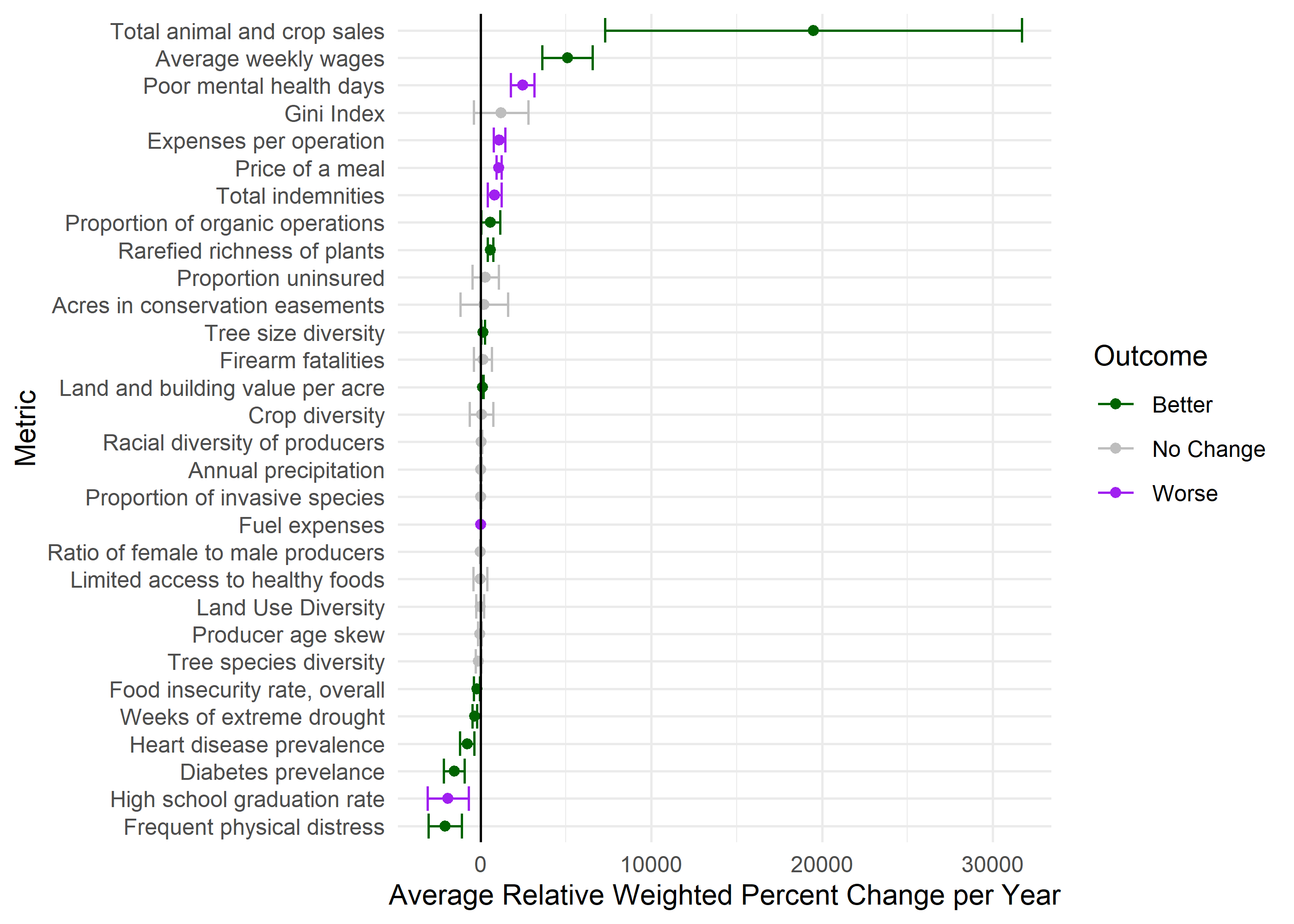
Issue here is that we have to drop many counties for some variables. The n column shows number of counties included. Some are well below half - not sure this is a great way to assess change if that is the case.
n: Number of counties included in regression
var: Metric
\(\rho\): Spatial autocorrelation in residual errors (omitted variables)
\(\beta\): Regression coefficient of year on the variable
se: standard error of \(\beta\)
t: test statistic
p-value: p-value
sig: whether p is < 0.05
reverse: whether the metric has been reversed so that lower numbers are better and higher numbers are worse (like food insecurity)
outcome: if the regression is significant, is it getting better or worse? Accounts for the ‘reverse’ variable